2. Materials and Methods
2.1. Chemicals and Reagents
The chemicals and reagents that were used in this study include; sulfuric acid (H2SO4, 98%, UNICHEM, Germany), nitric acid (HNO3, 69%, Loba Chemie Pvt. Ltd. India), hydrochloric acid (HCl, 35.4%, Loba Chemie Pvt. Ltd. India), potassium dichromate (K2Cr2O7, 99.5%, LABMERK CHEMICALS PVT. LTD. India), sodium chloride (NaCl, 99.9%, Fisher Chemical, US), sodium hydroxide (NaOH, 97% Loba Chemie Pvt. Ltd. India), potassium chromate (K2CrO4, Central Drug House (P) LTD, India), potassium dihydrogen orthophosphate (KH2PO4, 99%, Blulux Laboratories (P) Ltd. India), Violate Red Bile Agar (Central Drug House (P) Ltd. India), MacConky Agar (0.15%, HiMedia Laboratories Pvt. Ltd. India), Ammonium molybdate ((NH4)6Mo7O24, 98%, ALPHA CHEMICAL, India) and FAS ((NH4)2Fe(SO4)2·6H2O, 99%, Blulux Laboratories (P) Ltd. India).
2.2. Apparatus and Instruments
The materials required for this study were; beakers, flasks, pipette, measuring cylinders, spatulas, funnels, What man No 1 filter papers, desiccator, micropipettes, icebox, pH meter (Model: Bante902P, USA), Palin test photometer (Model: Palin test Photometer 7500, Germany), BOD incubator (Model: IN-010, GEMMYCO), mercury thermometer (Model 3012, UK), electronic balance (Model: JA103P, China), furnace (Model: SX-4-10, Drawell, China), oven (Model: GENLAB WLDNES, England), UV-Vis spectrophotometer (Model: SPECORD 200/PLUS, analytiKjena, Germany).
2.3. Study Area
Bedele Brewery Share Company was established on October, 1993 in Bedele town, located in the South Western part of Ethiopia’s Oromia Region, specifically in Buno Bedele Zone, Sadisa Keble. It is situated approximately 425 km away from Addis Ababa, the capital city of Ethiopia. As per annual report of Bedele Brewery in 2017, the company produces an impressive volume of 486,000 hectoliters (HL) of beer per year. In Bedele Brewery Share Company, some effluent (treated water) is reused in the company and the remaining effluent is discharged to the nearby Dabana river site, which can be the source of agricultural irrigation for the downstream farmers.
2.4. Sampling and Sample Points
The main source of the samples was water from the treatment plant system of the Bedele Brewery Share Company. Water samples were collected from two sampling points, i.e., one at influent (SP1) and the other at effluent (SP2) on March 1, 2025, for the first time and termed as day one (D1). The second time samples were taken on March 4, 2025, assigned as day two (D2) and the third time samples were taken on March 8, 2025 and termed as day three (D3). The sampling process and selection of sample points for water from a brewery treatment plant were conducted consistently over three days. On each day, duplicate samples were taken (i.e., 1 L at 9:00 AM in the morning and 1 L at 1:00 PM in the afternoon) and homogenized before analysis. The duplicate samples in the morning and afternoon for each day were mixed to ensure a representative sample. A time composite sampling method was used for the collection of water samples. Those sampling points were investigated to characterize its major parameters for the efficiency of the treatment plant as well as for the agricultural process. The collected samples were labeled and immediately transported in iceboxes to the Jimma University of Analytical Chemistry research laboratory for analysis.
2.5. Physiochemical Analysis of Samples
Some physical parameters such as total solids, total dissolved solids, total suspended solids, and volatile suspended solids were determined by the gravimetric method
| [14] | Kaur K. Handbook of Water and Wastewater Analysis; Atlantic Publishers & Dist, 2007. |
[14]
. Total solid (TS) concentration in the samples was determined by gravimetric method (Eq.
1) by pouring an aliquot of water sample into pre-weighed crucibles and subjected to heat in an oven at 180°C for 2 h. The residue was then cooled in the desiccator and weighed to a constant weight.
where TS is total solid (mg/L), W1 is weight of crucible in gram, W2 is weight of crucible with sample after drying in gram and V is sample volume.
The gravimetric method was used to quantify the total dissolved solids (TDS) in wastewater samples via Eq.
2. The first step was to weigh a clean crucible to a constant weight. The collected wastewater sample was then filtered into a clean conical flask. The filtrate was poured into the crucible in a volume of 10 mL. Afterwards, the crucible was dried at 180°C for 2 h. The residue was then cooled in a desiccator and weighed.
where TDS is total dissolved solid (mg/L), W
1 is weight of crucible only in gram, W
2 is weight of dried residue and crucible in gram and V is volume of sample in liter. Total suspended solid (TSS) was determined from the obtained values of TS and TDS via Eq.
3.
where TSS is total suspended solid in mg/L.
Volatile suspended solids (VSS) represent the fraction of TSS in a water sample consisting of living or deceased microorganisms and organic material. The VSS of sample was measured by Eq.
4 with taking of 10 mL of each sample underwent filtration, and the remaining material was moved to a crucible. The combined weight of the crucibles and the filter was noted as W
1. The crucible with the filter was then put in a muffle furnace at 550°C for 1.5 h to ensure full combustion of organic material. After cooling for 30 minutes in the desiccator to achieve room temperature and stable weight, the weight of the cooled crucible and residue was recorded as W
2.
where W1 is the weight of the crucible and filter before ignition (g), W2 is the weight of the crucible and residue after ignition (g) and V is the volume of the filtered sample (L). The temperature of sample was measured on the site of sample collection with mercury thermometer. The turbidity of water samples was determined by using palintest photometer. The pH of water samples was measured by a digital pH meter/multimeter. The Electrical conductivity of water sample was determined by the digital pH/multimeter.
The Mohr method, also known as the argentometric method, is a classic titrimetric technique for determining chloride (Cl
-) concentration in water samples. In this study the chloride content of samples was determined through Mohr method. The 50 mL of the samples were pipetted into the erlenmeyer flask and 3 drops of potassium chromate indicator solution was added to the flask, then the solution turned yellow. The burette was filled with 0.1N standard silver nitrate (AgNO
3) solution and the initial burette reading was recorded as V
1. On the continuously swirling flask, the sample was slowly titrated with the silver nitrate (AgNO
3) solution. The yellow color started to fade as silver chloride (AgCl) precipitate formed. Silver nitrate (AgNO
3) was continuously added to the endpoint of AgNO
3. The endpoint was indicated by a permanent brick-red color change in the solution and the final burette reading was recorded as V
2. Since 1 mole of Ag
+ reacts with 1 mole of Cl
- in the precipitation reaction, the moles of chloride ions in the sample are equal to the moles of silver ions used. So that the chloride content in samples was calculated by Eq.
5.
(5)
where M is molarity of silver nitrate (N), V
1 is initial burette reading in mL, V
2 is final burette reading in mL and V is volume of sample in mL
| [15] | Shukla M, Arya S. Determination of Chloride Ion (Cl-) Concentration in Ganga River Water by Mohr Method at Kanpur, India. Green Chemistry & Technology Letters 2018; 4: 6-8. |
[15]
.
The phosphate content of samples was determined via the spectrophotometric method through molybdate method. The molybdate method is a popular and established technique for determining phosphate concentration in wastewater due to its simplicity and affordability. The Vanadate-Molybdate Reagent was prepared by dissolving 0.1 g of ammonium metavanadate (NH
4VO
3) in 50 mL of 1:1 ratio HNO
3. Then 2.5 g of ammonium molybdate [(NH
4)
6Mo
7O
24]
was dissolved in 40 mL of distilled water in the beaker. The prepared reagent was transferred in to 100 ml volumetric flask water to the mark. The series of calibration standards were prepared from stock (1000 mg/L) potassium dihydrogen phosphate (KH
2PO
4). The prepared standard solutions were 0.1 mg/L, 0.5 mg/L, 1 mg/L, 1.5 mg/L, 2 mg/L, 2.5 mg/L, 3 mg/L and 10 mL of the vanadate-molybdate reagent was added to each standard solution. 25 mL of each sample was added in 50 mL volumetric flasks. 10 mL of the molybdate reagent was also added to each one and filled by distilled water to the mark. The all prepared solutions (including calibration standards) to be kept for 10 minutes until the full color was develop before taking absorbance readings. After the full color was developed the absorbance of each standard, sample and blank was measured at 470 nm. Finally the values of samples (i.e., influent and effluent) were determined from the calibration curve
| [16] | Adelowo FE, Oladeji SO. Spectrophotometric Analysis of Phosphate Concentration in Agricultural Soil Samples and Water Samples Using Molybdenum Blue Method. Brazilian Journal of Biological Sciences 2016; 3: 407-412. |
[16]
.
The chemical oxygen demand (COD) is an important parameter used to assess the amount of organic matter present in wastewater. The 25 mL of sample, 25 mL of oxidizing agent (i.e., 1000 mg/L K
2Cr
2O
7 were added in to the titration flask and 25 mL 0.5M H
2SO
4 was also added. The solution was mixed carefully and 3 drops of ferrion indicator was added and the solutions turn to greenish color. The titration was titrated against standard 0.5M ferrous ammonium sulfate (FAS) solution. This is back titrations, which gives the estimations of unreacted K
2Cr
2O
7 the solution and turns greenish to reddish brown when the end point was reached. For the estimations of the whole K
2Cr
2O
7 required for the experiment, blank titration was carried out through K
2Cr
2O
7, H
2SO
4 and ferrion of the same proportion in conical flask absence of the sample. The amount of COD in wastewater was calculated by using Eq.
6.
where A = volume of Mohr salt used for blank (L), B = volume of Mohr salt used for sample (L), C = normality of Mohr salt solution (eq/L) and V = volume of sample used (L)
| [17] | Agency USEP. Method 410.3: Chemical Oxygen Demand (Titrimetric, High Level for Saline Waters) by Titration; Office of Water Washington, DC, 1978. |
[17]
.
Biological oxygen demand (BOD) is a crucial parameter in assessing the organic pollution level of wastewater. It refers to the amount of dissolved oxygen (DO) needed by aerobic microorganisms to biodegrade organic matter in a water sample over a specific period and temperature. To ensure BOD content in the samples (i.e., 10 mL of the water sample was added in to two separate 300 mL BOD bottles). The initial DO concentration in each BOD bottle was measured using a Palin test and the value was record as DO
i. Each of BOD bottle then sealed tightly and incubated in the dark at 20 °C for 5 days. After 5 day, the final DO concentration in each bottle was measured using a Palin test and the value was record as DO
f. The blank control was prepared by filling a BOD bottle with dilution water only and treated identically to the samples. The final DO concentration in the blank control was measured and value was recorded as B
f. This accounts for any oxygen demand from the dilution water and seed culture. The BOD for each sample was calculated via Eq.
7.
(7)
where DO
i = Initial DO concentration in the sample bottle (mg/L), DO
f = Final DO concentration in the sample bottle (mg/L), B
f = Final DO concentration in the blank control (mg/L), V= volume of sample (mL) and volume of BOD bottle is also in mL
| [18] | Seif H, Malak M. Textile Wastewater Treatment Sixth International Water Technology Conference. IWTC, Alexandria, Egypt 2001. |
[18]
.
2.6. Biological Analysis of Samples
The serial dilution method is a common technique for quantifying total and fecal coliform bacteria in water. It involves diluting the water sample in a series of steps and testing each dilution to estimate the bacterial concentration per milliliter (mL). The series dilution of water sample was prepared through 10 mL of sample should be added to 10 mL of medium, 1 mL sample to 10 mL and 0.1 mL of sample to 10 mL of medium. By using micro-pipette 0.1 mL of each serial diluted solution was transferred to petri dishes containing MacConkey agar medium for fecal coliform and VRBA medium for total coliform. The inoculated samples in petri dishes was incubated at 37°C for 48 h and 44.5°C for 24 h for total coliform and fecal coliform respectively. After the incubation, the colonies on the agar mediums were counted. Colonies that are pink/red on MacConkey agar medium and red/pink on the VRBA medium indicates the existence of fecal coliform and total coliform respectively. The colony forming units (CFUs) per milliliter of the samples for both total coliform and fecal coliform was calculated based on the dilution factors and the number of colonies counted via Eq.
8.
(8)
where DF is dilution factor, CFU is colony forming unit CFU/mL.
2.7. Determination of Removal Efficiency
To assess the success of a treatment plant, it's crucial to perform a standard analysis of the wastewater and adhere to the proper procedures. This will allow for a determination of the treatment system's capacity and identification of any areas that require further examination. The removal efficiency of the effluent treatment plant for various wastewater quality parameters was determined via Eq.
9.
(9)
where Ci =the influent concentration of wastewater in mg/L and Ce= the effluent concentration of waste water in mg/L.
3. Result and Discussions
3.1. Physicochemical Analysis
The physicochemical parameters such as temperature, pH, EC, turbidity, TS, TDS, TSS, VSS, chloride, phosphate, BOD and COD contents of the treatment plant were determined.
3.1.1. Temperature Determination
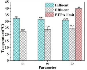
Figure 1. Temperature profiles of influent and effluent compared to EEPA limits, error bar indicates standard deviation.
Temperatures of water samples taken at the influent and the effluent were measured to check the effect brewery process on the heat content of water (
Figure 1). Accordingly, the mean temperature measurement of the influent was 32.40±0.26°C and ranged between 32.20 to 32.7°C while the mean temperature measurement of the effluent was 22.27±0.40°C and ranged between 21.9 to 22.7°C for D1. The mean temperatures of D2 and D3 for influent were 31.63±0.59°C and 30.99±0.16°C respectively. The mean temperatures of D2 and D3 for effluent were 23.91±1.47°C and 24.79±1.24°C respectively. Overall, the mean temperature values for the influent and effluent show variation across the three different days. The influent temperatures were relatively high, high rating need for temperature reduction during wastewater treatment. The effluent temperature consistently remained lower than the influent temperatures, indicating the effectiveness of the treatment process in reducing temperature. However, there were variations in the effluent temperature ranges indicates that, potential fluctuation in the treatment process or external factors impacting the temperature reduction. The temperature decrement in effluent was due to the flow wastewater through pipes and treatment units; it naturally loses heat to the surrounding environment. Both influent and effluent temperature values were within the natural brewery wastewater temperature (40°C) and possibly rising even higher.
3.1.2. pH Determination
pH is a significant factor in determining the acidity or alkalinity of water. In this study, the influent's average pH value was 9.22±0.01, while the effluent was 6.47±0.02 for D1. The mean pH of D2 and D3 for influent was 8.93±0.04 and 9.00±0.08 respectively (
Table 1). The effluent's D2 and D3 average temperatures were 6.72±0.91 and 6.64±0.20 respectively. As per
Table 1, the range of pH values for influent was between 9.21 to 9.23, and for effluent 6.46 to 6.50 for D1. The mean. pH values for the influent and effluent show slight variations across the three different days. The influent pH values were relativity high, indicating alkaline conditions in the presence calcium carbonates and other rocks. The effluent pH consistently decreased compared to the influent, indicating effective acidification or pH adjustment during the treatment process. However, there were variations in the effluent pH values, shows potential fluctuations in the treatment process or external factors impacting the pH adjustment. The pH values obtained for the effluent in this finding were within the acceptable range for brewery effluent discharge, which typically falls between 6 to 9.
Table 1. The pH profiles of influent and effluent compared with EEPA as well as WHO limit.
Parameter | pH values | EEPA limit | WHO limit |
D1 | D2 | D3 |
Influent | 9.22±0.01 | 8.93±0.04 | 9.00±0.08 | 6_9 | 6_9 |
Effluent | 6.47±0.02 | 6.72±0.91 | 6.64±0.20 |
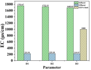
3.1.3. Electrical Conductivity Determination
Inorganic ions have a major influence on the conductivity of water. High values of EC show that inorganic ions are in abundance in the wastewater. EC is directly related to the concentration of dissolved ionized solids in water
| [19] | Al Dahaan S, Al Ansari N, Knutsson S. Influence of Groundwater Hypothetical Salts on Electrical Conductivity Total Dissolved Solids. Engineering 2016; 8: 823-830. |
[19]
. In essence, high EC in wastewater is an indication of high total dissolved solids concentration. The obtained EC mean value was 1753.67±1.53 μs/cm, 221.91±0.86 μs/cm; for influent and effluent respectively in D1. The mean EC for D2 and D3 for influent were 1722.33±3.06 μs/cm and 1689.83±2.90 μs/cm respectively. The average EC of effluent on D2 was 225.18±1.09 μs/cm while on D3 it was219.97±1.28 μs/cm. Over the three different days, there are only slight variations in the influent and effluent mean EC values. A significant electrical conductivity in the incoming water samples was indicated by the influent EC values, which were relatively high. When compared to the influent, the effluent EC consistently decreased indicating that the treatment process effectively reduced electrical conductivity. However, there were slight variations in the effluent EC values, implies the potential fluctuations in the treatment process or slight variations in the influent characteristics. The EC of influent value was above the discharge limit of EEPA, but the effluent value was lower than the discharge limit (
Figure 2). It was observed that EC decreased downstream and water does not contain excess dissolved salts that provide ions to conduct electricity and also the treatment plant was more effective EC removal.
Figure 2. The EC graph of influent and effluent compared to EEPA limits, error bar represents standard deviation.
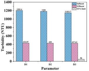
3.1.4. Turbidity Determination
Turbidity is commonly caused by the presence of clay, silt, organic matter, algae, and other microorganisms
| [3] | Fetaw AS, Haile MZ, Washe AP. Assessing the Chemical Composition of Wastewater Released from Hawassa Castel Brewery Plant and Its Impact on Groundwater. Journal of Waste Management & Xenobiotics 2021: 4. https://doi.org/10.23880/oajwx-16000164 |
[3]
. The mean value of turbidity was 1203.40±0.53 and 432.87±0.81 NTU for influent and effluent among the sampling stations respectively for D1. The average turbidity of influent on D2 was 1184.00±4.58, NTU while on D3 it was 1149.16±2.065 NTU. The average turbidity for D2 and D3 for effluent was 430.00±1.00 NTU and 427.00±0.65 NTU respectively (
Figure 3). The mean turbidity values of the influent and effluent exhibit fluctuations throughout the three different days. The influent turbidity values were relatively elevated, indicating the presence of suspended particles or cloudiness in the incoming water samples. The effluent turbidity consistently decreased compared to the influent, indicating a successful reduction of turbidity during the treatment process. Variations in the effluent turbidity values represent the possibility of fluctuations in the treatment process or variances in the characteristics of the influent. It was observed the result both influent and effluent data were above the EPA discharge limit of wastewater for irrigation
| [20] | EPA. Guidelines for Wastewater Irrigation and Land Application of Biosolids. 2012. |
[20]
.
Figure 3. Comparison of turbidity for industrial influent and effluent with EPA discharge limit, error bar indicates standard deviation.
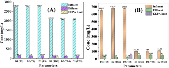
3.1.5. Gravimetric Analysis
Gravimetric analysis is a process used for determining the amount of a substance in a sample by measuring its mass. To carry out this type of analysis, it is important to obtain precipitates that are free of contaminants at a macroscopic level and can be easily filtered. The process of converting the analyte into sparingly soluble compounds of known composition, filtering, washing, and drying is called precipitation gravimetric analysis. Simple gravimetric analysis involves heating the sample, precipitating it, drying it, and separating it to determine the volatile and non-volatile components.
TS refer to all non-liquid matter that is either suspended or dissolved in wastewater. Wastewater that enters the treatment plant (also known as influent) typically has high TS due to the presence of industrial discharges. The TS value of effluent, was lower than the influent value because it undergoes primary treatment, which removes large settleable solids, secondary treatment, which reduces biological particles (especially organic matter), and tertiary treatment, which removes target-specific pollutants.
In this study, the TS value was 2751.67±2.89 mg/L for influent and 146.67±2.89 mg/L for effluent in D1. The average TS of influent on D2 was 2753.33±5.77 mg/L, while on D3 of it was 2751.66±2.89 mg/L. The average TS for D2 and D3 for effluent were 140.00±5.00 mg/L and 141.00±2.89 mg/L respectively (
Figure 4A). Across the three different days analyzed, the average amount of TS varied in both the influent and effluent. Influent TS levels were consistently high, signifying a substantial concentration of solids in the incoming wastewater. The effluent, however, displayed a consistent decrease in TS compared to the influent; emphasize that the treatment process effectively removes solids. However, some variation remained in the effluent's TS levels, which could be due to fluctuations in the treatment process itself or changes in the composition of the influent. The removal efficiency of TS for the company of D1, D2 and D3 was 94.67%, 94.92% and 94.85% respectively (
Table 3), which indicates that the treatment plant effectively remove TS from the wastewater. The TS removal efficiency of the company was higher than that of other brewery industries
| [21] | Daba C, Atamo A, Dagne M, Gizeyatu A, Adane M, Embrandiri A, Gebrehiwot M. Performance Evaluation of a Brewery Wastewater Treatment Plant in Ethiopia: Implications for Wetland Ecosystem Management. Lakes & Reservoirs: Research & Management 2022; 27: e12412. |
[21]
. The presence of this particular solid can have a negative impact on the environment by causing an increase in water cloudiness, a reduction in the amount of oxygen that is dissolved in the water, and harm to aquatic life. However, the results of the study show that the removal efficiency was quite high, and it was able to eliminate the more solid matter. This led to an effective treatment of the wastewater treatment plant.
TDS are inorganic salts and organic molecules that pass through the filter and remain dissolved in the wastewater. The removal efficiency of the plant for TDS of D1, D2 and D3 was 94.59%, 94.50% and 94.34% respectively. (
Table 3), which has mean values of influent 2093.33±5.77 mg/L and its corresponding effluent 113.33±5.77 mg/L in D1 respectively. The average TDS for D2 and D3 for influent were 2073.67±6.35 mg/L and 2073.00±4.36 mg/L respectively. The effluent's average TDS for D2 and D3 were 114.00±5.29 mg/L and 117.33±4.61 mg/L, respectively (
Figure 4A). The influent TDS concentrations were relatively similar on all three days, indicating consistent levels of dissolved solids in incoming water sample. The effluent TDS concentration also shows some similarity, with slight increase from D2 and D3. The removal efficiency of the treatment plant for TDS is very effective compared to other reported literature on brewery industries
| [2] | Firew T, Daniel F, Solomon SS. Performance Assessment of Wastewater Treatment Plant of Hawassa St. George Brewery, Hawassa, Ethiopia. Journal of Applied Sciences and Environmental Management 2018; 22: 1285-1292. |
| [21] | Daba C, Atamo A, Dagne M, Gizeyatu A, Adane M, Embrandiri A, Gebrehiwot M. Performance Evaluation of a Brewery Wastewater Treatment Plant in Ethiopia: Implications for Wetland Ecosystem Management. Lakes & Reservoirs: Research & Management 2022; 27: e12412. |
[2, 21]
. However the concentration of effluent was above the discharge limit of EEPA, which Is 80 mg/L; but below 133.5±34.3 mg/L reported in the other scholar
| [3] | Fetaw AS, Haile MZ, Washe AP. Assessing the Chemical Composition of Wastewater Released from Hawassa Castel Brewery Plant and Its Impact on Groundwater. Journal of Waste Management & Xenobiotics 2021: 4. https://doi.org/10.23880/oajwx-16000164 |
[3]
. So the study revealed that the treatment plant was more effective if the concentration of effluent below the discharge limit.
TSS determinations indicate the insoluble particles like sand, silt, organic matter, and algae that can be captured by a filter. The mean concentration of TSS in the influent was 658.33±7.64 mg/L. Similarly, the average concentration of TSS in the effluent was 33.33±5.29 mg/L for D1 and the average value TSS for D2, D3 for influent were 679.67±10.50 mg/L, 678.67±6.11 mg/L respectively. The effluent's average TSS for D2 and D3 were 26.00±1.72 mg/L and 24.33±4.04 mg/L respectively (
Figure 4B). The effluent TSS concentrations on D1 and D3 were lower than both the influent concentrations and the effluent concentrations on D1. This suggests that the treatment process effectively reduced the suspended solids in the water, resulting in improved water quality. The decreasing trend in effluent TSS concentrations over the three days indicates that the treatment plant process was consistently effective in removing suspended solids. The range of these values was between 650 to 665 for influent and 30 to 35 for effluent. Both influent and effluent value of TSS was lower than the results of previous study
| [22] | Choi HJ. Parametric Study of Brewery Wastewater Effluent Treatment Using Chlorella Vulgaris Microalgae. Environmental Engineering Research 2016; 21: 401-408. |
[22]
. The TSS concentration discharged into the open water was lower than the EEPA, 2003
| [23] | EEPA. Guideline Ambient Environment Standards for Ethiopia. Environmental protection authority and United Nations industrial development organization, Addis Ababa 2003; 1: 6-10. |
[23]
, which couldn’t affect the wetland ecological quality and biotic structure. The removal efficiency of the treatment plant of D1, D2 and D3 was 94.94%, 96.17% and 96.41% (
Table 3), which shows the plant effectively treat the concentration of TSS compared to other literature
| [2] | Firew T, Daniel F, Solomon SS. Performance Assessment of Wastewater Treatment Plant of Hawassa St. George Brewery, Hawassa, Ethiopia. Journal of Applied Sciences and Environmental Management 2018; 22: 1285-1292. |
| [21] | Daba C, Atamo A, Dagne M, Gizeyatu A, Adane M, Embrandiri A, Gebrehiwot M. Performance Evaluation of a Brewery Wastewater Treatment Plant in Ethiopia: Implications for Wetland Ecosystem Management. Lakes & Reservoirs: Research & Management 2022; 27: e12412. |
| [24] | Abrha BH, Chen Y. Analysis of Physico-Chemical Characteristics of Effluents from Beverage Industry in Ethiopia. Journal of Geoscience and Environment Protection 2017; 5: 172-182. |
[2, 21, 24]
.
VSS determination represents the organic fraction of TSS in wastewater. Understanding VSS concentration and characteristics is essential for effective sludge management, and nutrient loading assessment (i.e., it contributes to nitrogen and phosphorus loading in receiving water bodies, necessitating strategies to minimize nutrient discharge and protect water quality). The mean concentration value of VSS in the influent was found to be 103.33±5.74 mg/L and in the effluent was 54.00±5.29 mg/L for D1. The average value VSS for D2 and D3 for influent were 108.00±3.46 mg/L and 111.33±8.08 mg/L respectively. The effluent's average VSS for D2 and D3 were 56.33±4.72 mg/L and 53.00±4.36 mg/L, respectively (
Figure 4B). The effluent VSS concentrations for D2 and D3 were slightly higher than the effluent concentration on D1 but still lower than the influent concentrations for the respective days. This indicates that the treatment process was effective in reducing VSS. The result expresses that the treatment process generally succeeded in reducing VSS concentrations from the influent to the effluent. However, the slight increase in influent VSS concentrations over the three days and the variability in the effluent concentrations indicate the need for further investigation into the treatment process stability and performance. The range of these values was between 100 to 110 for influent and 52 to 60 for effluent. The concentration of influent was lower compared to the influent concentration other study (1799±57.1 mg/L) on the beer industry
| [25] | Khumalo SM, Bakare BF, Rathilal S, Tetteh EK. Characterization of South African Brewery Wastewater: Oxidation-Reduction Potential Variation. Water 2022; 14: 1604. |
[25]
. The removal efficiency of the treatment plant for VSS of D1, D2 and D3 was 47.74%, 47.99%, and 52.39% (
Table 3).
Figure 4. Gravimetric method result for TS, TDS, TSS & VSS and comparisons with EEPA limit, error bar indicates standard deviation.
3.1.6. Chloride Determination
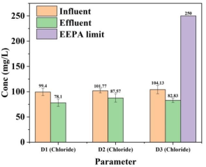
Figure 5. Chloride content representation of influent and effluent compared with EEPA limit, error bar shows standard deviation.
High levels of chloride in water inhibits the growth of plants, cause human illness, affect bacteria and fish in surface water and it can also lead to the breakdown in cell structure
| [26] | Chowdhury M, Mostafa MG, Biswas TK, Mandal A, Saha AK. Characterization of the Effluents from Leather Processing Industries. Environmental Processes 2015; 2: 173-187. |
[26]
. In present study the mean concentration of chloride ion in the influent was 97.03±4.10 mg/L and 78.10±7.1 mg/L for the effluent in D1 ranged between 92.30 mg/L to 99.40 mg/L of influent and 71.00 mg/L to 85.20 mg/L of effluent. The average value chloride for D2 and D3 for influent was 101.77±4.09 mg/L and 104.13±8.19 mg/L respectively. The effluent's average chloride for D2 and D3 were 87.56±8.19 mg/L and 82.83±4.09 mg/L, respectively (
Figure 5). The chloride concentrations in effluent for D2 and D3 were higher compared to D1, but the remained lower than the concentrations for the corresponding days. This indicates a certain level of effectiveness in reducing chloride ion through the treatment process. Overall, the results assert that the treatment process generally succeeded in reducing chloride ion concentrations from the influent to effluent. However, considering the slight increase in influent chloride concentrations over the three days and variability observed in the effluent concentrations, further investigation is necessary to assess the stability and performance of the treatment plant.
The removal efficiency of the treatment plant shows less effectiveness of chloride ion removing with the value of 19.51%, 13.95% and 20.46% for D1, D2 and D3 respectively (
Table 3). Even if, both influent and effluent values of chloride ion were below the discharge limit of EEPA, which is 250 mg/L
| [23] | EEPA. Guideline Ambient Environment Standards for Ethiopia. Environmental protection authority and United Nations industrial development organization, Addis Ababa 2003; 1: 6-10. |
[23]
. So that this study revealed that the requirement of raw materials to generate the chloride ion in the beer processing of the company is low.
3.1.7. Phosphate Determination
Phosphate is an essential nutrient for plant and especially important in water pollution because they are effective nutrient sources for algae (organic phosphorus converted to inorganic phosphate). Excessive presence of phosphate in water causes algal blooms which result in the death of aquatic organisms
| [27] | Bhateria R, Jain D. Water Quality Assessment of Lake Water: A Review. Sustainable Water Resources Management 2016; 2: 161-173. |
[27]
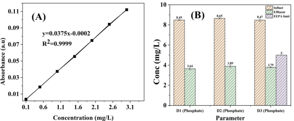
. In this study the phosphate level in influent and effluent were determined by spectroscopic method of calibration curve (
Figure 6A). The mean concentration value of phosphate in the influent was 8.49±0.06 mg/L and 3.64±0.09 mg/L in effluent for D1 with the range value between 8.45 mg/L to 8.53 mg/L for influent and 3.57 mg/L to 3.71 mg/L effluent. The average value phosphate ions for D2 and D3 for influent were 8.65±0.06 mg/L and 8.47±0.13 mg/L respectively. The effluent's average values of phosphate ions for D2 and D3 were 3.89±0.11 mg/Land 3.78±0.04 mg/L, respectively (
Figure 6B).
The treatment process effectively reduced phosphate levels in the effluent compared to the influent for overall three days. However, D2 and D3 shows slightly higher effluent concentrations compared to D1, indicating some variability in removal efficiency. Additionally, it is noteworthy that the influent phosphate levels have somewhat decreased during the course of the days. Overall, the data evinces a generally successful treatment for phosphate removal, but further investigation is needed to optimize stability and consistency. The removal efficiency of phosphate ion from the wastewater of the company was 57.14%, 55.03%, and 55.25% for D1, D2, and D3 respectively (
Table 3), which less effective compared to other brewery wastewater treatment plant of phosphate ion
| [28] | Angassa K, Assefa B, Kefeni KK, Nkambule TT, Fito J. Brewery Industrial Wastewater Treatment through Mesocosm Horizontal Subsurface Flow Constructed Wetland. Environment Systems and Decisions 2022; 42: 265-275. |
[28]
. The concentration of after treatment plant was lower than the EEPA, which is 5 mg/L as well as the reported values in the other literature
| [3] | Fetaw AS, Haile MZ, Washe AP. Assessing the Chemical Composition of Wastewater Released from Hawassa Castel Brewery Plant and Its Impact on Groundwater. Journal of Waste Management & Xenobiotics 2021: 4. https://doi.org/10.23880/oajwx-16000164 |
| [28] | Angassa K, Assefa B, Kefeni KK, Nkambule TT, Fito J. Brewery Industrial Wastewater Treatment through Mesocosm Horizontal Subsurface Flow Constructed Wetland. Environment Systems and Decisions 2022; 42: 265-275. |
[3, 28]
.
Figure 6. Calibration Curve (A) and comparison of phosphate concentration with EEPA limit (B), error bar indicates standard deviation.
3.1.8. Biochemical Oxygen Demand Determination
BOD is the amount of oxygen utilized by microbial organisms to decompose organic compounds in water. BOD test is used to determine the extent of pollution of a wastewater and the efficacy of effluent treatment methods. DO is greatly influenced by the BOD level in water. The higher BOD concentration, the greater extent of oxygen depletion in the water bodies. This results in the reduction of oxygen available for higher forms of aquatic life which consequently leads to the death of aquatic organisms
| [27] | Bhateria R, Jain D. Water Quality Assessment of Lake Water: A Review. Sustainable Water Resources Management 2016; 2: 161-173. |
[27]
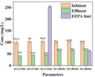
. The percentage removal of the treatment plant for BOD of D1, D2 and D3 was 35.39%, 35.66% and 33.70% (
Table 3) respectively. The concentration of BOD of the influent and effluent were found to be 99.60±0.85 mg/L and 64.35±0.64 mg/L respectively in D1 with value of influent was ranged between 99.00 mg/L to 100.20 mg/L and 63.90 mg/L to 64.80 mg/L for effluent. The influent average BOD was 103.05±1.06 mg/L on D2 and 98.55±0.21 mg/L on D3, with minimal day-to-day variation. The effluent average BOD was 66.30±0.85 mg/L on D2 and 65.25±0.42 mg/L on D3 (
Figure 7). The treatment process significantly reduced BOD in the effluent compared to the influent for all three days. D2 and D3 showed slightly higher effluent levels than D1. This demonstrates some variability in treatment efficiency. The minimal day-to-day variation in influent BOD indicates a consistent source of organic pollutants. Overall, the data suggests a generally effective treatment process for BOD removal, but further investigation is needed to optimize its stability and consistency. The value of both influent and effluent concentration was did not comply with EEPA, which is 60 mg/L
| [23] | EEPA. Guideline Ambient Environment Standards for Ethiopia. Environmental protection authority and United Nations industrial development organization, Addis Ababa 2003; 1: 6-10. |
[23]
. The effluent value and removal efficiency was lower compared to reported values in the other scholars of brewery wastewater
| [2] | Firew T, Daniel F, Solomon SS. Performance Assessment of Wastewater Treatment Plant of Hawassa St. George Brewery, Hawassa, Ethiopia. Journal of Applied Sciences and Environmental Management 2018; 22: 1285-1292. |
[2]
. So that the treatment plants requires other treatment methods, that adds the BOD removal efficiency and lowers the effluent concentrations from the limit value. So the water has high content of organic matter and has counts of microbial organisms.
3.1.9. Chemical Oxygen Demand Determination
COD is the measure of oxygen equivalent of the organic content of the sample that is susceptible to oxidation by a strong chemical oxidant. It is an evaluation used to measure the level of water contamination by organic matter
| [29] | Alrumman S, Keshk S, El Kott A. Water Pollution: Source & Treatment. American Journal of Environmental Engineering 2016; 88-98. |
[29]
. The COD value was higher than the BOD because some organic materials in the water that are resistant to microbial oxidation and hence not involved in BOD could be easily chemically oxidized. The COD of influent was 101.33±9.24 mg/L and effluent was 42.67±9.24 mg/L in D1. The average value COD for D2 and D3 for influent were 104.00±8.00 mg/L and 104.53±8.05 mg/L respectively. The effluent's average values of COD for D2 and D3 were 45.33±4.62 mg/L and 46.4±2.77 mg/L, respectively (
Figure 7).
The COD concentrations in the effluent on D2 and D3 were slightly more than on the D1, although they were still far lower than the amounts in the influent on those days. Even though the results varied a little, this suggests that the treatment method was successful in lowering organic contaminants. The treatment process proved generally successful in lowering COD concentrations from the influent to the effluent, which led to a significant decrease in organic pollutants. Organic contaminants are consistently input, as indicated by the small daily change in influent COD values. The variation in the effluent concentrations and the requirement for further investigation into the effectiveness and stability of the treatment process should be observed. The measured value of COD was below the effluent standard limit value of beverage industries; which is of 250 mg/L
| [23] | EEPA. Guideline Ambient Environment Standards for Ethiopia. Environmental protection authority and United Nations industrial development organization, Addis Ababa 2003; 1: 6-10. |
[23]
. It also revealed that the COD concentration effluent value was lower than the COD concentration of brewery industries by other scholars
| [24] | Abrha BH, Chen Y. Analysis of Physico-Chemical Characteristics of Effluents from Beverage Industry in Ethiopia. Journal of Geoscience and Environment Protection 2017; 5: 172-182. |
[24]
. Results obtained after treatment gave 52.38% in D1, 56.41% in D2, and 55.61% in D3 reduction efficiency for COD levels of the treatment plant (
Table 3), which was not effective compared to other study with removal efficiency of 96.7% for COD
| [21] | Daba C, Atamo A, Dagne M, Gizeyatu A, Adane M, Embrandiri A, Gebrehiwot M. Performance Evaluation of a Brewery Wastewater Treatment Plant in Ethiopia: Implications for Wetland Ecosystem Management. Lakes & Reservoirs: Research & Management 2022; 27: e12412. |
[21]
.
Figure 7. Comparison of BOD and COD with their corresponding EEPA limit, error bar indicates standard deviation.
3.2. Total and Fecal Coliform Determination
The biological parameters such as total coliforms and fecal coliforms of the treatment plant were analyzed. Testing for fecal coliforms involves inoculation of MacConkey agar followed by incubation at 44.5 °C for 24 h. Growth accompanied by development of red colonies are considered to be positive results for MacConkey agar. Fecal coliforms are involved in food spoilage and cause illness in both humans and animals
| [30] | Patel AK, Singhania RR, Pandey A, Joshi VK, Nigam PS, Soccol CR. Enterobacteriaceae, Coliforms and E. Coli. In Encyclopedia of Food Microbiology: Second Edition; Elsevier Inc., 2014; pp 659-666. |
[30]
. The Violet Red Bile Agar (VRBA) medium was used as a selective medium for the identification of total coliform by incubation at 37 °C for 48 h. Total and fecal coliforms were isolated from influent and effluent. As shown in
Table 2, the total coliform per samples spreading on VRBA ranged from 1.94*10
5CFU/100 mL to 1.95*10
5CFU/100 mL and 9.5*10
4CFU/100 mL to 9.56*10
4CFU/100 mL for influent and effluent respectively for D1. The fecal coliform numbers in influent grow on MacConkey agar ranged from 5.5*10
4CFU/100 mL to 5.62*10
4CFU/100 mL and effluent of ranged from 2.0*10
4CFU/100 mL to 2.01*10
4CFU/100 mL for D1. The total coliform of influent for D2 and D3 were ranged between 1.845*10
5CFU/100 mL to 1.85*10
5CFU/100 mL and 1.998*10
5CFU/100 mL to 2.0*10
5CFU/100 mL respectively. The total coliform of effluent for D2 and D3 were ranged between 8.49*10
4CFU/100 mL to 8.5*10
4CFU/100 mL and 9.0*10
4CFU/100 mL to 9.11*10
4CFU/100 mL respectively. The fecal coliform of influent for D2 and D3 were ranged between 6.0*10
4CFU/100 mL to 6.14*10
4CFU/100 mL and 5.0*10
4CFU/100 mL to 5.12*10
4CFU/100 mL respectively. The fecal coliform of effluent for D2 and D3 were ranged between 2.45*10
410
4CFU/100 mL to 2.5*10
4CFU/100 mL and 1.44*10
4CFU/100 mL to 1.5*10
4CFU/100 mL respectively. The presence of coliform bacteria was confirmed in the water samples. Influent counts remained consistent across the three days, similar to both total and fecal coliform counts. While the treatment process appears to reduce coliform bacteria (due to lower effluent counts compared to influent), some variability in effluent counts requires further investigation of the treatment plant.
Table 2. Summary of total coliform and fecal coliform for the influent and effluent compared with WHO.
Parameters | Day | Samples and No of colonies (103) | Mean of CFU (CFU/100mL) | Log (CFU) | WHO limit |
Influent | Effluent | Influent | Effluent | Influent | Effluent |
Total coliform (TC) | 1 | 19.50 | 9.50 | 1.95*105 | 9.5*104 | 5.29 | 4.98 | 1 |
2 | 18.50 | 8.50 | 1.85*105 | 8.5*104 | 5.27 | 4.9 |
3 | 20.00 | 9.00 | 2*105 | 9*104 | 5.3 | 4.95 |
Fecal coliform (FC) | 1 | 5.50 | 2.00 | 5.5*104 | 2*104 | 4.74 | 4.3 |
2 | 6.00 | 2.50 | 6*104 | 2.5*104 | 4.78 | 4.39 |
3 | 5.00 | 1.50 | 5*104 | 1.5*104 | 4.67 | 4.18 |
3.3. Wastewater Treatment Plant Efficiency
The performance of the Bedele Brewery wastewater treatment plant was evaluated on the basis of its removal efficiency of major parameters including; temperature, pH, turbidity, EC, TS, TDS, TSS, VSS, Cl
-, PO
43-, BOD, COD, TC and FC as shown in the (
Table 3). The removal efficiency of the treatment plant was effective for the removal of TS, TDS, TSS and EC. The treatment plant has high efficiency for TS, TDS, TSS and EC, with compared to others scholar report on brewery treatment of TS, TDS, TSS and EC; 65.5%, 70.2%, 57.2% and 29.1% respectively
| [21] | Daba C, Atamo A, Dagne M, Gizeyatu A, Adane M, Embrandiri A, Gebrehiwot M. Performance Evaluation of a Brewery Wastewater Treatment Plant in Ethiopia: Implications for Wetland Ecosystem Management. Lakes & Reservoirs: Research & Management 2022; 27: e12412. |
[21]
. Effective removal of organic compounds from wastewater is important to avoid anaerobic conditions in receiving waters
| [31] | Driessen W, Vereijken T. Recent Developments in Biological Treatment of Brewery Effluent. In The Institute and Guild of Brewing Convention, Livingstone, Zambia, March; Citeseer, 2003; pp 2-7. |
[31]
. However, the removal efficiency of BOD (35.39%) and COD (52.38%) from the wastewater of the treatment plant was less effective compared to previous study with BOD 96% and for COD 92%
| [2] | Firew T, Daniel F, Solomon SS. Performance Assessment of Wastewater Treatment Plant of Hawassa St. George Brewery, Hawassa, Ethiopia. Journal of Applied Sciences and Environmental Management 2018; 22: 1285-1292. |
[2]
.
Table 3. Overall pollutant removal efficiency of the treatment plant.
Parameters | Mean ± STD values | Removal efficiency (%) | EEPA limit |
Influent | Effluent |
D1 | D2 | D3 | D1 | D2 | D3 | D1 | D2 | D3 |
Temp (°C) | 32.40±0.26 | 31.63±0.59 | 30.99±0.16 | 22.27±0.04 | 23.91±1.47 | 24.79±1.24 | 31.27 | 24.41 | 20.01 | 40 |
pH | 9.22±0.01 | 8.93±0.04 | 9.01±0.08 | 6.47±0.02 | 6.72±0.19 | 6.64±0.21 | 29.79 | 24.75 | 26.22 | 6-9 |
Turbidity (NTU) | 1203.40±0.53 | 1184.00±4.58 | 1149.16±2.065 | 432.87±2210.81 | 430.00±1.00 | 427.00±0.65 | 63.03 | 63.73 | 62.79 | |
EC (μs/cm) | 1753.67±1.53 | 1722.33±3.06 | 1689.83±2.90 | 221.91±0.86 | 225.18±1.09 | 219.97±1.28 | 87.35 | 86.93 | 86.98 | 1000 |
TS (mg/L) | 2751.67±2.89 | 2753.33±5.77 | 2751.66±2.89 | 146.67±2.89 | 140.00±5.00 | 141.00±2.89 | 94.67 | 94.92 | 94.85 | |
TDS (mg/L) | 2093.33±5.77 | 2073.67±6.35 | 2073.00±4.36 | 113.33±5.77 | 114.00±5.29 | 117.33±4.61 | 94.59 | 94.50 | 94.34 | 80 |
TSS (mg/L) | 658.33±7.64 | 679.67± 10.50 | 678.67±6.11 | 33.33±2.87 | 26.00±1.72 | 24.33±4.04 | 94.94 | 96.17 | 96.41 | 50 |
VSS (mg/L) | 103 33±5.74 | 108.00±3.46 | 111.33±8.08 | 54.00±5.29 | 56.33±4.72 | 53.00±4.36 | 47.74 | 47.99 | 52.39 | |
Cl- (mg/L) | 97.03±4.10 | 101.77±4.09 | 104.13±8.19 | 78.10±7.10 | 87.56±8.19 | 82.83±4.09 | 19.51 | 13.95 | 20.46 | 250 |
PO43- (mg/L) | 8.49±0.06 | 8.65±0.06 | 8.47±0.13 | 3.64±0.09 | 3.89±0.11 | 3.78±0.04 | 57.14 | 55.03 | 55.25 | 5 |
BOD (mg/L) | 99.60±0.85 | 103.05±1.06 | 98.55±0.21 | 64.35±0.64 | 66.30±0.85 | 65.25±0.42 | 35.39 | 35.66 | 33.79 | 60 |
COD (mg/L) | 101..00±40.00 | 104±8.00 | 104.53±8.05 | 42.67±9.24 | 45.33±4.62 | 46.40±2.77 | 52.38 | 56.41 | 55.61 | 250 |
TC (CFU/mL) | 1.95*105±707.10 | 1.85*105±353.55 | 2*105±141.42 | 9.5*103±424.26 | 8.5*103±70.71 | 9*103±777.82 | 51.28 | 54.05 | 55.00 | < 1 |
FC (CFU/mL) | 5.5*103±848.52 | 6*104±989.94 | 5*104±848.52 | 2*104±70.71 | 2.5*104±353.55 | 1.5*104±424.26 | 63.64 | 58.33 | 70.00 | < 1 |
3.4. Effluent Suitability for Agricultural Irrigation
Brewery effluent, the wastewater generated during beer production, presents a potential source of irrigation water. However, its suitability depends on various factors, including its composition, treatment processes, and local regulations. Based on the provided parameters, the Bedele Brewery effluent exhibits both promising and concerning aspects for agricultural irrigation. The temperature falls within the typical range for brewery effluent (
Table 4) and is not expected to pose significant concerns for irrigation unless combined with other unfavorable factors
| [20] | EPA. Guidelines for Wastewater Irrigation and Land Application of Biosolids. 2012. |
[20]
. The pH value of effluent was slightly acidic and within the acceptable range for irrigation (
Table 4) according to EPA guidelines
| [20] | EPA. Guidelines for Wastewater Irrigation and Land Application of Biosolids. 2012. |
[20]
. However, it is important to monitor pH closely as acidic effluent can acidify soil over time, impacting nutrient availability and plant growth. Turbidity significantly higher than the recommended limit (
Table 4) for irrigation water (50 NTU)
| [20] | EPA. Guidelines for Wastewater Irrigation and Land Application of Biosolids. 2012. |
[20]
, indicating the presence of suspended solids. High turbidity can clog irrigation systems (i.e., hindering water distribution and potentially damaging equipment), reduce light penetration in soil (i.e., impacting plant growth and beneficial microorganisms), and potentially harbor pathogens like bacteria and coliforms present in the effluent. Further treatment is necessary to reduce turbidity before using this effluent for irrigation. According to EPA guidelines for the brewing industry does not specify a limit for EC. However, elevated salinity levels in irrigation water can affect soil structure, water uptake, and crop growth (
Table 4).
The TS of present study was (142.55±3.59 mg/L), TDS was 114.89±5.22 mg/L and TSS was 27.89 ± 2.87 mg/L (
Table 4), while the guideline of EPA doesn't provide a direct limit for TS, TDS and TSS in brewery effluent. However, high levels of solids can clog irrigation systems and affect soil structure. High TSS levels can be problematic for irrigation by clog irrigation systems (i.e., hindering water distribution and potentially damaging equipment), reduce light penetration in soil (i.e., impacting plant growth and beneficial microorganisms) and harbor pathogens if they contain organic matter or microorganisms. Proper treatments, such as sedimentation of filtration, required to reduce solid content. The EPA guidelines for brewing industry recommended a maximum VSS limit of 20 mg/L for wastewater discharges
| [20] | EPA. Guidelines for Wastewater Irrigation and Land Application of Biosolids. 2012. |
[20]
. The provided VSS (54.44 ±4.79 mg/L) level exceed this limit (
Table 4), indicating a need for adequate treatment to reduce VSS content before using the effluent for agricultural irrigation. Excessive amounts of VSS can deplete soil oxygen, hindering root development and beneficial microbial activity, contribute to odors as well as create nuisance conditions.
The EPA does not specify a limit for chloride in brewery effluent. However, high chloride levels can be harmful to sensitive crops and affect soil fertility (
Table 4). The EPA guidelines for the brewing industry do not provide specific limits for phosphate ion (
Table 4). However, excessive phosphate levels can lead to eutrophication of water bodies. Nutrient management practices should be implemented to prevent nutrient imbalances in soil and water bodies. The BOD (65.30±0.63 mg/L) and COD (44.8±5.54mg/L) indicate potentially excessive organic matter (
Table 4). While some is beneficial, too much can deplete soil oxygen (i.e., hindering root development and beneficial microbial activity), contribute to odors and create nuisance conditions. Adequate treatment processes like advanced oxidation should be applied to reduce organic pollutants before using the effluent for irrigation. The levels of total coliform (9*10
4±424.26CFU/mL) and fecal coliform (2*10
4±282.84CFU/mL) significantly exceed acceptable limits for irrigation water, posing a significant health risk. So proper treatment, such as disinfection, would applied to ensure microbial safety before using the effluent for irrigation.
Table 4.
Suitability of Bedele Brewery effluent for agricultural irrigation purpose compared to EPA guideline | [20] | EPA. Guidelines for Wastewater Irrigation and Land Application of Biosolids. 2012. |
Parameters | Effluent values | EPA Guideline for Irrigation Water | Suitability for Irrigation |
Temperature (°C) | 24.41±0.04 | No specific limit | Acceptable |
pH | 6.61±0.02 | 6.0 - 8.5 | Acceptable, but monitor closely |
Turbidity (NTU) | 429.95±0.81 | < 50 | Highly unsuitable, requires significant treatment |
EC (μs/cm) | 222.53±0.86 | Site-specific based on soil properties and crop tolerance | Requires further analysis of ionic composition for salinity assessment |
TS (mg/L) | 142.55±2.89 | No set restriction | Depending on certain constituents, monitoring can be necessary |
TDS (mg/L) | 114.89±5.77 | No specific limit | May require monitoring depending on specific constituents |
TSS (mg/L) | 27.89±2.87 | No specific limit, but high levels can impact irrigation systems | Contributes to high turbidity, requires treatment |
VSS (mg/L) | 54.44±5.29 | 20 | Part of total suspended solids, contributes to organic matter content |
Cl- (mg/L) | 82.83±7.10 | Site-specific depending on crop tolerance and soil characteristics | Potentially concerning for salt-sensitive plants, requires further analysis |
PO43- (mg/L) | 3.77±0.09 | No specific limit, but can contribute to nutrient loading | Beneficial depending on crop needs and soil nutrient status |
BOD (mg/L) | 65.3±0.64 | No set limit | Requires treatment to reduce oxygen demand in soil |
COD (mg/L) | 44.8±23.09 | No specific limit, but high levels indicate organic matter overload | Has to be treated in order to lower oxygen demand in soil |
TC (CFU/mL) | 9*104±353.55 | < 2 per 100 mL | Highly unsuitable, poses significant health risk |
FC (CFU/mL) | 2*104±141.42 | < 1 per 100 mL | Extremely inappropriate and dangerous for one's health |