Abstract
The location, design, drilling and completion of wells for potable groundwater abstraction require exploration and mapping of groundwater potential zones within the geologic framework of any region. In this study, field data acquisition involved seven vertical electrical sounding and three horizontal resistivity profiling (HRP) carried out. Field data were interpreted using IPI2win 1-D software while subsurface lithologic layering and correlation was realized in rockworks v 22. Modelled true geolectric sections after curve matching revealed the study area to be underlain predominantly by clayey lithologic units followed by coarse grained sands with silty sands and fine sands in minor fraction. Total investigation depth range between 314.0m and 510.0m and fresh water was found to occur at a depth of 168m in VES L2, 430m in VES L3 and 154m in VES L6 locations. Iron water was found in some coarse sands at a depth interval of 129 m to 314 m at VES L1 while fresh water in coarse sands underlain by iron water saturated fine sands occurs at a depth interval of 73.20 m to 206 m at VES L2. At VES L3, fresh water saturated coarse sands were found at a depth interval of 131 m to 430m. Boreholes should be drilled to 430m and screened from 131m to 430m at L3. At VES L4, fine sands overlying coarse grained sands were saturated with iron water from 50.20 m to 422m. At VES L6, fresh water saturated coarse grained sandy aquifer was found from 114 m to 154m. Although VES L2, L3 and L6 provides the most suitable prospective locations for fresh water in the area at depths of 168m for L2, 430m for L3 and 154m for L6, lithologic modelling revealed that both coarse sands and fine sands are either juxtaposed or interfingered at the shallow, intermediate and deeper depths, hence, there is strong potential for iron water and fresh water inter-mixing during pumping. All twenty proposed boreholes are recommended not to be pumped at rates exceeding 3,500 l/min. Boreholes should be 450m apart to prevent well interferences and pumping schedule of 10 to 14 boreholes daily will greatly reduce stresses on the well field as well as potential risk from saline intrusion. Three saline water encroachment monitoring boreholes should be sited at 1.5km from L1 and L2 and 2.4km from L7 respectively at the East, West and Southern sections of the plant area.
Keywords
Groundwater Potential Zones, Geoelctric Layers, Fresh Water, Salt Water Intrusion
1. Introduction
The coastal Niger Delta is industrializing rapidly and population growth is rising exponentially due to migration to the oil rich region. Water is vital and essential for manufacturing and production operations
| [1] | Than, N. N., Thunyawatcharakul, P., Ngu, N. H. and Chotpantarat, S. (2022). Global review Global review of groundwater potential models in the last decade: Parameters, model techniques, and validation. Journal of Hydrology, Volume 614, Part A, November 2022, 128501. |
[1]
and human occupancy in any region also requires considerable amounts of water of desirable quality to meet the demands of domestic uses and industrial applications. Due to long term oil and gas exploration and production activities in the Niger Delta region, hydrocarbon transporting pipelines rupture causing point source release of contaminants of concern into the surface water bodies, soil and groundwater, nearly all the water sources are heavily polluted. Coastal aquifer salinization by salt enriched intra-formation trapped seaward marine deposits, fossil sea water, leaching from saline confining beds, saline sea water intrusion, increase in the total dissolved solids, and tidally induced enlargement of salt water zones
| [2] | Abija, F. A., Abam, T. K. S., Teme, S. C. and Eze, C. L. (2011). Relative Sea Level Rise, Coastline Variability and Coastal Erosion in the Niger Delta, Nigeria: Implications for Climate Change Adaptation and Coastal Zone Management. J. Earth Science and Climate Change vol., 11:9, pp. 1–10. FOR code: 240504. |
[2]
remain a fundamental consideration in every groundwater planning and design in the region. This is exacerbated by climate change induced eustatic sea level rise in addition to the subsidence induced relative rise in sea level currently affecting the region
| [3] | Abija, F. A., Harry, I. M. and Udom, G. J. (2020). Sources of Salinization and Investigation of Salt Water Intrusion into Coastal Aquifers in Parts of the Niger Delta, Nigeria. Journal Hydrogeology and Hydrologic Engineering, vol., 9:4, pp. 1–8. |
[3]
. This causes onshore migration of the freshwater/saltwater interface in accordance with the Ghyben – Herzberg principle
| [4] | Baydon-Ghyben, W. (1889). Nota in verban met de voorgenomen putboring nabij Amsterdam., Koninlyk Instituut Ingennieurs Tidjchrift (The Hauge) 1888 – 1889, pp. 8–22. |
| [5] | Herzberg, A. (1901). “Die Wasserversorgung einiger Nordseebader”. Journal Gasbeleuchtung und Wasserversorgung (Munich), 44(1901), 815–19, 842-44. |
[4, 5]
and further engendering lateral and depth-wise extension of the interface. Atmospheric pollution by flue gas (soot) also renders rain water harvesting non-usable, thereby forcing an almost complete reliance on groundwater to meet domestic and industrial needs in the Niger Delta region.
The geology of the Niger Delta brings nearly all surface-water features (streams, lakes, reservoirs, wetlands, and estuaries) into interaction with groundwater
| [6] | Abam, T. K. S. and Nwankwoala, H. O. (2020) Hydrogeology of Eastern Niger Delta: a Review. Journal of Water Resource and Protection, 2020, 12, 741-777. |
[6]
. These interactions are most evident in the many coastal islands in the Niger Delta and take many forms. In some situations, surface-water bodies gain water from groundwater systems and in others the surface-water body is a source of groundwater recharge and causes changes in groundwater quality as well. At deeper levels (deep borehole prospects >150m depth), the quality of groundwater in the Niger Delta closely follows the sedimentation pattern
| [7] | Ngah, S. A. and Nwankwoala, H. O. (2013) Assessment of Static Water Level Dynamics in Parts of the Eastern Niger Delta. The International Journal of Engineering and Science, 2, 136-141. |
[7]
. Based on water quality
| [6] | Abam, T. K. S. and Nwankwoala, H. O. (2020) Hydrogeology of Eastern Niger Delta: a Review. Journal of Water Resource and Protection, 2020, 12, 741-777. |
[6]
, subdivided the Eastern Niger Delta into 3 distinct groundwater zones; The continental deposits of the Northern Border; the Transition Zone, and; the Mangrove Swamp land areas. The present study area lies within the mangrove swamp land areas where significant iron contamination has been reported for deep aquifer prospects
| [8] | Ngah S. A (2009) Deep Aquifer Systems of Eastern Niger Delta: Their Hydrogeological Properties, Groundwater Chemistry and Vulnerability to Degradation, PhD Thesis, Rivers State University, Port-Harcourt, Nigeria. |
[8]
. The iron is commonly in the form of ferrous iron which generally remains in solution when water samples are freshly collected. However, upon exposure to the atmosphere, the ferrous iron comes in contact with oxygen in the atmosphere and is oxidized into its ferric equivalent which is generally brownish in colour. The acidic nature of groundwater, characterized by low pH ensures that iron and manganese remain in solution, both of which impart an unpleasant and unpalatable taste. The source of the iron contamination has been a subject of debate but it is suggested to have been emplaced by iron fixing bacteria associated with sedimentary environments of decaying vegetative matter. The exposure of quaternary sediments to glaciation was accompanied by eustatic lowering of the sea level such that could expose the sediments to the oxygen rich atmosphere and created paleo-soils rich in iron oxides
| [9] | Abam, T. K. S. (2001). Regional hydroiogical research perspectives in the Niger Delta. Hydroiogical Sciences- Hydroiogical Sciences-,)'ouriwl-des Sciences Hydrologiques, 46(1), pp. 13-32. |
[9]
. The subsequent rise in sea level would have incorporated the paleo-soils into the geologic record. Hence, this is the reason for significant iron content in groundwater sources around the study area. Also, the rate of movement and circulation of groundwater in deeper horizons greatly decreases due to significantly reduced hydraulic gradients. This in turn implies greater retention times which would allow more minerals to be dissolved so that concentration tends to increase with depth. This process can lead to a vertical stratification, with bicarbonates predominant in the upper zone and chlorides at depth
| [10] | Edwards, K. A., Classen, G. A. and Schroten, E. H. J. (1983) The Water Resource in Tropical Africa and Its Exploitation. E-Book Series. ILCA Publications, 103 p. |
[10]
. Hence, this is the reason for significant iron content in groundwater sources in the region. Therefore, identifying prospective groundwater zones is crucial for planning and design of abstraction wells; and for resource conservation and management.
The siting and drilling of boreholes for groundwater abstraction requires pre-drilling well design assessment to determine the potential and potability of the resource. Groundwater potential refers to the total amount of permanent storage that exists in the aquifers. It denotes storage, transmission and flow into abstraction tube wells
| [11] | Abija, F. A., Essien, N. U., Abam, T. K. S and Ifedotun, A. I. (2019). Assessment of Aquifer Hydraulic Properties, Groundwater Potential and Vulnerability Integrating Geoelectric Methods with SRTM -DEM and LANDSAT -7 ETM lineament Analysis in Parts of Cross River State, Nigeria. London Journal of Research in Science: Natural and Formal, Volume 19 | Issue 7 | Compilation 1.0, pp. 35–51. |
[11]
and quantifies the tendency of water to move from one area to another due to osmosis, gravity, mechanical pressure and matrix effects such as capillary
. Groundwater potential is a function of porosity and permeability and the driving impetus for groundwater flow is the force potential which is equivalent to the product of the hydraulic head and the gravitational acceleration as noted by
| [13] | Fetter CW (1988) Applied hydrogeology, 2nd edn. CBS Publishers, New Delhi. |
[13]
. Groundwater potential can be measured by (a) recharge rate and mechanism, (b) aquifer storage and transmission properties, and (c) suitability of the water from water quality point of view and (d) the response of the aquifer to changes such as climate, seasonality, artificial withdrawal and pollution
| [14] | Kebede, S. (2013). Groundwater Potential, Recharge, Water Balance: Vital Numbers. In: Groundwater in Ethiopia. Springer Hydrogeology. Springer, Berlin, Heidelberg. |
[14]
. Groundwater yield and abstraction in wells depends on the position, thickness and lithology of the reservoir and confining beds as well as the hydraulic characteristics of the aquitards and aquifers alike; and the amount of groundwater withdrawal. Groundwater potential zone refers to subsurface reservoirs with adequate porosity, permeability, storage of groundwater resources of good quality and would permit its flow into an abstraction well in quantity to support pumping. Hydrological factors often used in groundwater potential evaluation include geology, slope, land use, soil type, drainage density, lineament density, altitude, rainfall
| [1] | Than, N. N., Thunyawatcharakul, P., Ngu, N. H. and Chotpantarat, S. (2022). Global review Global review of groundwater potential models in the last decade: Parameters, model techniques, and validation. Journal of Hydrology, Volume 614, Part A, November 2022, 128501. |
[1]
. Groundwater potential zones are the objective target of hydrogeological investigations for sustainable water management to meet the water needs of various sectors such as drinking water, agriculture, and industry. Assessment of groundwater potential has been achieved using invasive methods
| [15] | Ugbaja, A. N., William, G. A. and Ugbaja, A. A. (2021). Evaluation of groundwater potential using aquifer characteristics on parts of boki area, south – eastern nigeria. Global journal of geological sciences vol. 19, 2021: 93-104. |
| [16] | Zhang, Z. Zhang, S., Li, M. Zhang, Y., Chen, M., Zhang, Q. Dai, Z. and Liu, J. (2023). Groundwater Potential Assessment in Gannan Region, China, Using the Soil and Water Assessment Tool Model and GIS-Based Analytical Hierarchical Process. Remote Sens., 15(15), 3873. |
| [17] | Yohana, A. R., Makoba, E. E., Mussa, K. R., Mjemah, I. C. (2023). Evaluation of Groundwater Potential Using Aquifer Characteristics in Urambo District, Tabora Region, Tanzania. Earth 2023, 4(4), 776-805. |
[15-17]
non-invasive methods using geophysical techniques
| [18] | Ehirim, C. N. and Nwankwo, C. (2016) Quality Assessment and Evaluation of Groundwater Potentials in Parts of Buruku and Gboko Local Government Area Councils in Benue State. International Journal of Geosciences, 7, 1064-1073. |
| [19] | Aizebeokhai, A. P., Oyeyemi, K. D. and Joel, E. S. (2016). Groundwater potential assessment in a sedimentary terrain, southwestern Nigeria. Arab J Geosci (2016) 9:496 pp. 2–15. |
| [20] | Alabi, A. A., Popoola, O. I., Olurin, O. T. et al. Assessment of groundwater potential and quality using geophysical and physicochemical methods in the basement terrain of Southwestern, Nigeria. Environ Earth Sci 79, 364 (2020). |
| [21] | Ekwok, S. E., Akpan, A. E., Kudamnya, E. A. and Ebong, E. D. (2020). Assessment of groundwater potential using geophysical data: a case study in parts of Cross River State, south eastern Nigeria. Applied Water Science (2020) 10: 144. |
| [22] | Arafa, S. A. S., Hamed, H., Nayef, A., Sabet, H. S., AbuBakr, M. M., and Mebed, M. E. (2023). Assessment of groundwater aquifer using geophysical and remote sensing data on the area of Central Sinai, Egypt. Scientifc Reports | (2023) 13:18245, pp. 1–18. |
| [23] | Ubaidullah, A., Francis, A. A. and Francis, W. K. (2021). Assessment of groundwater potential using vertical electric sounding technique at Faculty of Medicine and Engineering, Federal University Dutsin-ma Katsina State, Nigeria. Global Journal of Earth and Environmental Science Volume 6(4), pages 98-105. |
| [24] | Li, K., Yan, J., Li, F., Lu, K., Yu, Y., Yulin Li, Y. Zhang, L., Wang, P. Li, Z., Yang, Y. and Wang, J. (2014). Non invasive geophysical methods for monitoring the shallow aquifer based on time lapse electrical resistivity tomography, magnetic resonance sounding, and spontaneous potential methods. Scientifc Reports | (2024) 14:7320, pp. 1-12. |
| [25] | Raji, W. O. and Abdulkadir, K. A. (2023). Evaluation of groundwater potential of bedrock aquifers in Geological Sheet 223 Ilorin, Nigeria, using geo electric sounding. Applied Water Science (2020) 10:220 pp. 1-12. |
[18-25]
, geographic information systems and remotely sensed data
| [26] | Duguma, T. A. and Duguma, G. A. (2022). Assessment of Groundwater Potential Zones of Upper Blue Nile River Basin Using Multi-Influencing Factors under GIS and RS Environment: A Case Study on Guder Watersheds, Abay Basin, Oromia Region, Ethiopia. Geofluids Volume 2022, Article ID 1172039, pp 1–26. |
| [27] | Boitt, M., Khayasi, P. and Wambua, C. (2023) Assessment of Groundwater Potential and Prediction of the Potential Trend up to 2042 Using GIS-Based Model and Remote Sensing Techniques for Kiambu County. International Journal of Geosciences, 14, 1036-1063. |
| [28] | Tamesgen, Y, Atlabachew, A. and Jothimani, M. (2023). Groundwater potential assessment in the Blue Nile River catchment, Ethiopia, using geospatial and multi-criteria decision-making techniques. Heliyon 9 (2023) e17616 pp. 1–21. |
| [29] | Opoku, P. A.; Shu, L.; Amoako-Nimako, G. K. (2024). Assessment of Groundwater Potential Zones by Integrating Hydrogeological Data, Geographic Information Systems, Remote Sensing, and Analytical Hierarchical Process Techniques in the Jinan Karst Spring Basin of China. Water 2024, 16, 566. |
[26-29]
. There is a paucity of groundwater potential studies in Ikot Abasi area even though studies abound
| [18] | Ehirim, C. N. and Nwankwo, C. (2016) Quality Assessment and Evaluation of Groundwater Potentials in Parts of Buruku and Gboko Local Government Area Councils in Benue State. International Journal of Geosciences, 7, 1064-1073. |
| [19] | Aizebeokhai, A. P., Oyeyemi, K. D. and Joel, E. S. (2016). Groundwater potential assessment in a sedimentary terrain, southwestern Nigeria. Arab J Geosci (2016) 9:496 pp. 2–15. |
| [21] | Ekwok, S. E., Akpan, A. E., Kudamnya, E. A. and Ebong, E. D. (2020). Assessment of groundwater potential using geophysical data: a case study in parts of Cross River State, south eastern Nigeria. Applied Water Science (2020) 10: 144. |
[18, 19, 21]
in other parts of the basin.
This study was aimed at identifying and mapping suitable groundwater horizons for sustainable long-term use for industrial as well as domestic utilization of coastal areas. The objectives include conducting on-site non-intrusive geophysical studies to determine lithological sequence of sediments and establish the presence and depth to potable groundwater, determination of subsurface stratigraphic units, delineation of aquifers subsurface stratigraphic intervals, identification of best locations for drilling water supply boreholes. determination of adequate borehole drill depth, provide insights into the subsurface aquiferous system, detection of depth to saline water at survey points., generate subsurface ground models of the study area to characterize aquifers in terms of thickness, water quality and long-term sustainability and create groundwater surface response to pumping using characteristic hydraulic parameters of the area.
2. Study Area
2.1. Location and Climate
The study area is located in Okopedi Community of Ikot Abasi L.G.A. of Akwa Ibom State. The coastal area is bounded geographically by Latitudes 4°28'6.84"N and 4°31'21.29"N and Longitudes 7°34'13.09"E and 7°39'58.69"E of the Greenwich meridian.
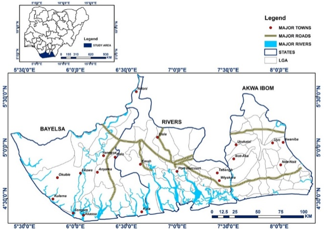
Figure 1 is a map of the project site, highlighting areas for infrastructure, creek, swamps and River networks along with surrounding vegetation. It is located on the south-western part of Akwa Ibom State. The Imo River forms the natural boundary in the east separating Studied site’s plot area from Rivers State. The area is that of humid tropic with the temperature range of 26°C and 28°C, while the mean annual rainfall lies between 2,000-4,000 mm. The rainy season lasts from April to November and is characterized by high relative humidity and heavy cloud covers. However, the region is endowed with enormous natural resources. It has the world’s third largest mangrove forest with the most extensive freshwater swamp forest and tropical rainforest characterized by great biological diversity. The topography of the area is gently undulating with a relief ranging from 2.0m to 3.50m above mean sea level. The project site can be assessed mainly through the Ikot-Abasi-Eket Expressway. Located at the north of the area is Okoro Iyong community, Imo River to the west, Qua Iboe River to the east and Ikomata community and the Atlantic Ocean to the South of the area.
Figure 1. Map of parts of the Niger Delta showing the study area.
There are several networks of creeks and swamp inlets within the area. Due to the coastal nature of the area, most of the creeks and swamps are currently been closed up in order to reclaim significant land area for utilization.
2.2. Regional Hydrogeological Setting
The Niger Delta geology is underlain by three principal formations, namely: Akata, Agbada and Benin Formations. The hydrogeology of the Niger delta is dominated by the Benin Formation, which serves not only as aquifer but also facilitates recharge of groundwater in the region. The Benin Formation serves as the groundwater reservoir in Ikot Abasi. The main body of groundwater in the Niger Delta is contained in the extensive sand and gravel layers which are interspersed with shale and clay layers within the formation. It is now well known that the Benin Formation (Miocene to Recent) posses’ excellent water yielding properties even at great depths
| [30] | Amajor, L. C. (1991) Aquifers in the Benin Formation (Miocene-Recent) Eastern Niger Delta, Nigeria: Lithostraigraphy, Hydraulics and Water Quality. Environmental Geology and Water Sciences, 17, 85-101. https://doi.org/10.1007/BF01701565 |
[30]
. Well cuttings from the logs of oil wells spread across the Niger delta, reveal that the Benin Formation is laterally extensive and extends to depths of 2000 m in places
| [6] | Abam, T. K. S. and Nwankwoala, H. O. (2020) Hydrogeology of Eastern Niger Delta: a Review. Journal of Water Resource and Protection, 2020, 12, 741-777. |
[6]
.
| [31] | Etu-Efeotor, J. O. and Odigi, M. I. (1983). Water Supply Problems in the Niger Delta. J. of Mining and Geology, vol. 20 (1&2), pp. 183–193. |
| [32] | Akpokodje, E. G., Etu-Efeotor, J. O. and Mbeledogu, I. U. (1996) A Study of Environmental Effects of Deep Subsurface Injection of Drilling Waste on Water Re- sources of the Niger Delta. CORDEC, University of Port Harcourt, Port Harcourt. |
| [33] | Akpoborie, I. A. (2011) Aspects of the Hydrology of the Western Niger Delta Wetlands: Groundwater Conditions in the Neogene (Recent) Deposits of the Ndokwa Area. Proceedings of the Environmental Management Conference, Federal University of Agriculture, Abeokuta, 13 p. |
[31-33]
’s studies indicate that the Benin Formation is differentiated into three main zones, namely; (1) a northern bordering zone consisting of shallow aquifers of predominantly continental deposit, (2) a transition zone of intermixing marine and continental materials and (3) a coastal zone of predominantly marine deposits.
| [32] | Akpokodje, E. G., Etu-Efeotor, J. O. and Mbeledogu, I. U. (1996) A Study of Environmental Effects of Deep Subsurface Injection of Drilling Waste on Water Re- sources of the Niger Delta. CORDEC, University of Port Harcourt, Port Harcourt. |
[32]
summarized the hydrostratigraphic units of the Benin Formation as consisting of four well defined aquifers in the upper 305 m that vary in thickness. The aquifers vary from unconfined conditions at the surface through semi-confined to confined conditions at depth. The aquifers are separated by highly discontinuous layers of shales, giving a picture of an interval that consists of a complex, non-uniform, discontinuous and heterogeneous aquifer system. In 2014, an estimated groundwater recharge of 31.9 BCM/year was predicted by Japan International Cooperation Agency for the Niger delta region of Nigeria. This value is just below that of the South East region which is the highest in Nigeria. The high perennial aquifer recharge in the area is supported by the abundant rainfall averaging 2,532 mm/year, favorable geology, vast catchment area, North Southwards groundwater flow and presence of a rich network of fresh water rivers and streams in the area.
3. Materials and Methods
The present study utilizes non-intrusive scientific approaches to gain better understanding of the subsurface aquifer system, determine suitable targets for producing potable groundwater, understand potential impacts that may arise from long-term aquifer production, determine potential of salt intrusion from surrounding creeks and address the groundwater recovery sources and mechanisms impact of the boreholes in the communities around the project site. Static water level measurements were carried out in available boreholes in an area. The geophysical method employed is the Vertical Electrical Sounding (VES) resistivity method. The choice of this method was based on the fact that the target of interest (groundwater) is depth driven (600 m). Both Wenner and Schlumberger resistivity method were selected. A total of seven (7) resistivity lines were run across the project area. Of the seven lines run, four (4) were run using the Schlumberger array while three (3) survey lines were run using the Wenner array. The purpose of electrical surveys is to determine the subsurface resistivity distribution by making measurements on the ground surface. From these measurements, the true resistivity of the subsurface can be estimated. The ground resistivity is related to various geological parameters such as the mineral and fluid content, porosity and degree of water saturation in the rock. Electrical resistivity surveys have been used for many decades in hydrogeological and geotechnical investigations. In Okopedi, the lack of potable water supply has led to very few boreholes installed in the area. Borehole installations identified are greater than 3.0km away from available facility in the study area. Also, all boreholes (3 boreholes) identified were cased and installed with locked well heads hence, there was no means of measuring the static water level from surrounding boreholes. The static water level measurements obtained from Vertical Electrical Sounding resistivity investigations for the unconfined aquifers are 1.38m, 1.44m, 4.46m, 0.94m, 3.69, 2.86m and 4.80m for VES points L1, L2, L3, L4, L5, L6 and L7 respectively. These results are expected considering the close proximity of the area to the coastline. Generally, the static water level in the area ranged from 0.94m at VES point L4 and 4.80m at VES point L7 respectively. Generally, groundwater flow direction across the Niger Delta area is from the North towards the South
| [33] | Akpoborie, I. A. (2011) Aspects of the Hydrology of the Western Niger Delta Wetlands: Groundwater Conditions in the Neogene (Recent) Deposits of the Ndokwa Area. Proceedings of the Environmental Management Conference, Federal University of Agriculture, Abeokuta, 13 p. |
| [6] | Abam, T. K. S. and Nwankwoala, H. O. (2020) Hydrogeology of Eastern Niger Delta: a Review. Journal of Water Resource and Protection, 2020, 12, 741-777. |
[33, 6]
. Meanwhile, in the north-east (Imo River catchment area) which includes the study area Okopedi, groundwater flow is from the northeast towards the southwestern area into the Imo River
| [6] | Abam, T. K. S. and Nwankwoala, H. O. (2020) Hydrogeology of Eastern Niger Delta: a Review. Journal of Water Resource and Protection, 2020, 12, 741-777. |
[6]
. Seasonal variations have a huge impact on the level of groundwater in the subsurface. During rainy season, there is a significant rise in the water table elevation and a significant decline in the water table during the dry season. Even coastal aquifers experience these impacts although at a much-decreased rate.
| [7] | Ngah, S. A. and Nwankwoala, H. O. (2013) Assessment of Static Water Level Dynamics in Parts of the Eastern Niger Delta. The International Journal of Engineering and Science, 2, 136-141. |
[7]
reported groundwater decline in shallow and deep aquifers to range from 1.40m to 6.0m. The smaller drops (1.40m) were associated with shallow aquifers while the more significant drops (6.0m) were associated with deep aquifers in the Niger Delta. This suggests a maximum of 6.0m drop in water levels in boreholes proposed to be drilled within studied site (impact from seasonal variations).
3.1. Survey Design
The goal of the project was to identify deep potable groundwater prospects at depths up to 600m. To achieve the project’s objectives, seven (7) VES points were selected across the entire study area. The area is swampy and most of the creeks located within the industrial area of the study site prevented accessibility at the time of this survey, hence, some of the survey lines run were repositioned. Also, to achieve a depth of investigation of 600m, the total lengths of survey lines on the surface needs to extend for 3,000m (Wenner array) and 2,500m (Schlumberger array). The project area has a dimension of 4000 m x 2000 m; hence, survey lines were extended beyond the industrial site in order to get significant investigation depth.
Figure 2 is a map of the study area, showing both orientation and length of the VES survey lines run across the project area.
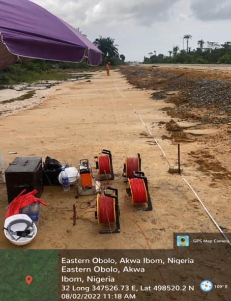
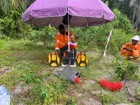
Table 1 shows the geographic reference coordinates, line orientation, elevation and length of each survey line run. Areas where the proposed lengths of survey lines were not achieved were as a result of inaccessibility due to creeks or swamps. In this study, the vertical electrical sounding (VES) technique was employed to delineate potential groundwater-bearing zones. The Vertical Electrical Sounding survey is based on the principle that allows the passage of current into the ground by means of current electrodes and measuring the potential drop between potential electrodes. Current penetrates into the ground with increase in electrodes spacing. In a ground consisting of different lithology with depth, apparent resistivity is measured where the pattern of current flow is influenced by the density, porosity and salinity of the contained fluid in the ground. Both Schlumberger and Wenner arrays were employed in this study. The Wenner array configuration with a maximum half current electrode separation of 1500 m was adopted for survey Line 1, Line 2 and Line 3, while the Schlumberger array configuration with a maximum half current electrode separation of 1200 m was adopted for VES Line 4, Line 5, Line 6 and Line 7. The main advantage of using the Schlumberger array configuration is because it requires fewer electrodes to be moved for each sounding, gives better vertical resolution and has greater probing depth (Keary and Brooks, 1984). The Schlumberger array consists of four collinear electrodes separated from each other by some known distance. The outer two electrodes are the current electrodes and the inner ones are the potential electrodes. An ABEM SAS 1000 resistivity meter was used to measure the apparent resistivity at each survey station. At every sounding point, the potential electrodes were planted at the middle of the electrode array with the electrode spacing less than one fifth of the spacing between the current electrodes. The current electrodes were moved at different distances whilst keeping the potential electrodes constant until the voltage became too small to measure before the potential electrodes were increased accordingly. The Wenner array configuration was also utilized. The challenge with the Wenner array configuration is that it requires a lot of man power, it is more stressful to conduct and requires more space to achieve same investigation depth achieved while using the Schlumberger array configuration. The outer two electrodes are the current electrodes and the inner ones are the potential electrodes. An ABEM SAS 1000 resistivity meter was also used to measure the apparent resistivity at each VES station. At every sounding point, all current and potential electrodes were placed equidistant from each other (
figures 2 and 3) are site photographs taken during geophysical investigation).
Figure 2. Vertical Electrical Sounding resistivity survey along Station L2.
Figure 3. Vertical Electrical Sounding resistivity survey along Station L6.
During data acquisition, certain precautions were taken in order to ensure the acquired results are representative.
1) Four (4) measurement cycles were set on the ABEM SAS 1000 Terameter so as to acquire sufficient results (thousands of resistivity values for a given spread) for averaging.
2) Results with high standard deviation (>8%) were rejected and re-run so as to ensure the results obtained are representative of the formation.
3) Although the area is very swampy, where possible, hard grounds were always selected for pinning electrodes into the ground to allow for sufficient soil area to have contact with the electrodes.
4) Due to the long line lengths (half current electrode spread of 1500 m), survey lines were carefully marked out using ropes and caution tapes prior to commencement of survey. Geographic reference coordinates of the ends of each line from the midpoint were determined before survey so as to validate and correct any curved lines.
5) Four (4) 12 volts’ batteries were taken to the project site daily to prevent shortage of power. While sounding deeper depth targets (> 250 m), charged batteries were used in order to allow sufficient current to travel significant depths into the subsurface. Low batteries were never used to sound deep depth targets.
6) Measurements were repeated severally in order to ensure the integrity of the results.
7) Daily equipment calibration checks were done by acquiring resistivity values within a known vicinity (an area where the resistivity values are already known) prior to commencement of work on site.
8) Transmitted current from ABEM SAS 1000 Terameter was set at 1000 mA (automatic). With these settings, the ABEM SAS 1000 Terameter run preliminary tests and then selects the most appropriate current to transmit into the subsurface. Deeper depth targets require more current be transmitted because some of the current will be naturally attenuated with depth.
Table 1. Geographic coordinates, line length and orientation of VES survey lines.
Line No. | Current Electrode End (C1) | Midpoint | Current Electrode End (C2) | Line Orientation | VES method | Length of Line |
Coordinates (UTM 32N) | Elevation (m) | Coordinates (UTM 32N) | Elevation (m) | Coordinates (UTM 32N) | Elevation (m) |
Line 1: | E345063 | 5.00 | 346460 | 5.00 | 347852 | 5.00 | E-W | Wenner | 2,760m |
N497838 | 497896 | 497935 |
Line 2: | E344390 | 6.00 | 345653 | 7.50 | 346970 | 7.00 | NW-SE | Wenner | 2,760m |
N500017 | 499596 | 499151 |
Line 3: | E348022 | 4.00 | 347048 | 5.50 | 346064 | 6.00 | NE-SW | Wenner | 2,400m |
N498481 | 497820 | 497200 |
Line 4: | E346306 | 5.00 | 347272 | 6.00 | 348258 | 6.00 | NE-SW | Schlumberger | 2,400m |
N497555 | 498255 | 498953 |
Line 5: | E344451 | 4.00 | 345174 | 4.80 | 345890 | 5.00 | NNW-SSE | Schlumberger | 2,300m |
N497433 | 496612 | 495782 |
Line 6: | E343789 | 7.00 | 344927 | 8.55 | 346111 | 8.21 | NW-SE | Schlumberger | 2,400m |
N499906 | 499620 | 499298 |
Line 7: | E345505 | 5.00 | 346676 | 4.33 | 347858 | 5.00 | NW-SE | Schlumberger | 2,400m |
N497156 | 496907 | 496663 |
3.2. Data Processing and Analysis
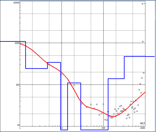
A maximum current of 1000 mA was selected for the survey using an automatic approach. The ABEM SAS 1000 Terameter tests various currents and selects the most suitable current for investigating various depths. This process led to acquisition of data with acquisition error below 5%. High errors are mainly caused by insufficient current utilized during data acquisition. High errors are reduced during data acquisition by using an automatic approach for selecting most suitable current for investigations. Apparent resistivity values are obtained by multiplying the acquired resistance with the geometric factor for a given electrode spread. Field data were recorded on site and plotted on a graph of apparent resistivity against half-electrode spacing using a bi-logarithmic graph. The generated VES curves were smoothened in order to ensure that all the effects of lateral inhomogeneity and other forms of noisy signatures were minimized. Acceptable readings were obtained at a maximum standard deviation of 8.0%. The higher standard deviations were recorded at greater depth (> 300m depth). Depths shallower than 300m all had standard deviation error below 2.0%. At every station, the field resistance data were converted to apparent resistivity by multiplying the resistances by the equivalent geometric factor. The final computed apparent resistivity data was processed using the IPI2win 1-D inversion software. Data imported into the inversion software includes electrode spacing, geometric factor and apparent resistivity. The data is coded in a format readable by the processing software. Upon import of the data, a graph is generated with Apparent resistivity on the Y-axis and Current electrode spread on the X-axis. The graph shows a plot of the calculated apparent resistivity against the current electrode spacing. Scatter points on the graph are the apparent resistivity values. The blue line shows layer thicknesses while the red curve is the ideal theoretical curve used for curve matching. Embedded within the theoretical field curve are geoelectric layer properties which includes true resistivity of the formation, the thickness of the formation and the depth to each layer. During data processing, the ideal theoretical field curve is adjusted to match with the acquired field apparent resistivity data. As the adjustments are made to the ideal theoretical curve, new soil layers are added to improve the adjustment. A good adjustment (good fit between ideal theoretical curve and field apparent resistivity data) is obtained when the root mean square error is below 15% and the interpretations are geologically realistic. The final inverted resistivity model provided information about the true resistivity of layers, their thicknesses, and depths of occurrence. In this study, the data fit was maintained at a reasonable root mean square error (RMS) values of 5-19%. The root mean square is a measure of the closeness of the theoretical curves to the observed field curves as the manual adjustment was done to get the best fit. There are two major assumptions which must be known while using the VES method; (1) Each modelled layer is assumed to be homogenous based on acquired resistivity values, (2) Each layer is assumed to be horizontal and laterally continuous. It should be known that apparent resistivity acquired from the field undergoes processing which converts the results to true resistivity of the formations. The actual investigation depth is only known after successfully processing the acquired apparent resistivity measurements. Results obtained from data processing were then analyzed and made ready for interpretation. The true resistivity of each soil layers was assigned geological interpretations based on published standards and guidelines and also based on known geological settings of the area. The thickness and depths of each soil layer obtained after inversion were used to plot geoelectric sections for the various survey sounding points. Each layer was then interpreted based on the true resistivity of the soil layer, the depth to each soil layer and the thickness of each soil layer.
3.3. Lithologic Modelling
RockWorks 22 software program was used for creating 2-D and 3-D maps, logs, cross sections, development of geological models, lithologic and stratigraphic modelling. The choice of rockworks for this study was based on its vast applicability in groundwater modelling globally, its relative ease of use and ability to generate quick interactive maps easy to evaluate and remodel without having to re-run the entire simulation process as required by other modelling software. The process involves populating interpreted lithologies and associated depths within the borehole manager interface. The softwares utilizes complex geostatical algorithms in development of lithologic models from borehole data.
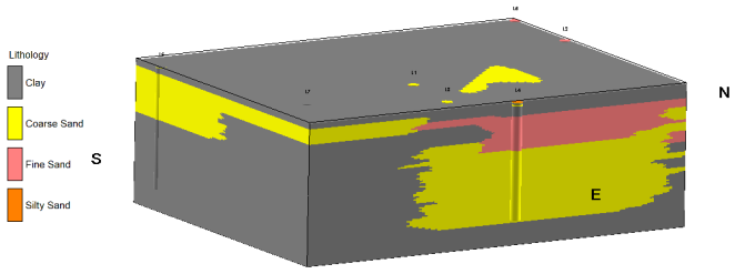
Figure 18 shows a 3-D grid generated after interpolation of all borehole lithologic data. The lithologies revealed are mainly clay, followed by coarse sand, fine sand and silty sand. The fence diagrams presented in
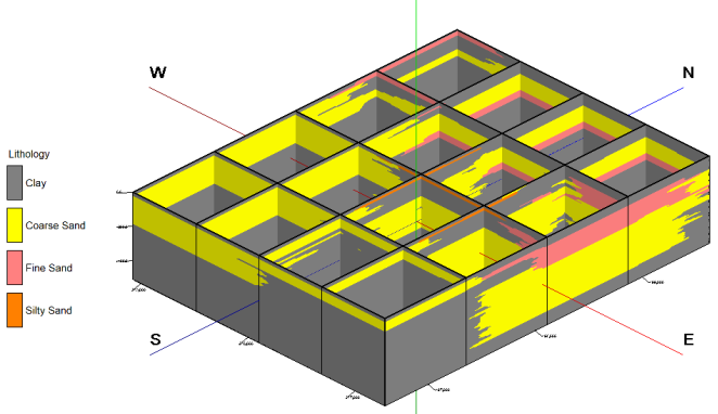
Figures 11, 12 and 13 shows strong inter-connectivity between the shallow aquiferous sands and the deep groundwater aquifers. The profile lines (
Figures 20, 21, 22, 23) shows strong connectivity between shallow aquiferous sands and iron water rich sands at both shallow and deeper depths. Although shales abound at the top and bottom of all lithologic units, their distribition appears fairly more continuous across the area. The connectivity observed within the sandy units and the silty sandy units across all survey points suggest the tendency for continuous communication between the shallow and deeper aquifer porospects.
4. Presentation of Results
4.1. Vertical Electrical Sounding Lines
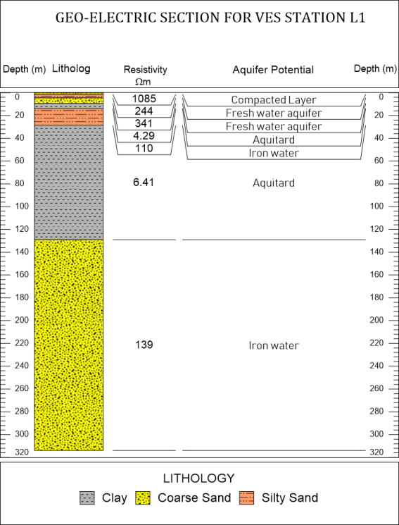
Figures 4-17 shows the VES modelled curves and their respective interpreted geolectric layers for all sounding locations in the project area. These properties aid in the selection of viable groundwater drill targets within studied site. Lithologic attributes including true resistivity of the formation, depth and thickness or each resistivity layer are embedded in the ideal theoretical curve. During data processing, matching the acquired apparent resistivity values with the ideal field curve modifies the geoelectric properties of the rock layers and in many cases, additional geoelectric layers are added for a good representative match with reduced error. RMS error represents residual difference between actual field measurements and the ideal theoretical curve after matching both data. Seven geo-electric layers were modelled from VES Line 1 (
Figure 4 and
figure 5). Layer 1 extends from 0.0m at the surface to 1.38m depth. The layer has a thickness of 1.38m and a representative resistivity value of 1085 Ωm. The layer has been interpreted as coarse grained sand. The high resistivity values recorded for this interval suggest the absence of a fluid phase due to the compacted nature of the soils as a result of ongoing road construction around this point. The second geo-electric layer extends from 1.38 m to 4.56 m depth. The layer has a thickness of 3.18 m and a representative resistivity value of 244 Ωm. The layer has been interpreted as fresh water silty sand. Hence, this layer has good aquifer potential. The third geo-electric layer extends from 4.56 m to 9.43 m depth. The layer has a thickness of 4.87 m and a representative resistivity value of 341 Ωm. The layer has been interpreted as fresh water coarse sand. Hence, this layer has an excellent aquifer potential. The fourth geo-electric layer extends from 9.43 m to 13.90 m depth. The layer has a thickness of 4.47 m and a representative resistivity value of 4.29 Ωm. The layer has been interpreted as a clayey unit with no aquiferous potential. The fifth geo-electric layer extends from 13.90 m to 28.60 m depth. The layer has a thickness of 14.70 m and a representative resistivity value of 110 Ωm. The layer has been interpreted as a silty sandy unit bearing iron water. This layer has been interpreted as having fair aquifer potential. This is because iron water is not potable and needs to be treated prior to consumption. The sixth geo-electric layer extends from 28.60 m to 129 m depth. The layer has a thickness of 100.40 m and a representative resistivity value of 6.41 Ωm. This thick layer has been interpreted as a clayey unit with no aquiferous potential. The seventh geo-electric layer extends from 129 m to 314 m depth. The layer has a thickness of 185 m and a representative resistivity value of 139 Ωm. The layer has been interpreted as a coarse sandy unit bearing iron water.
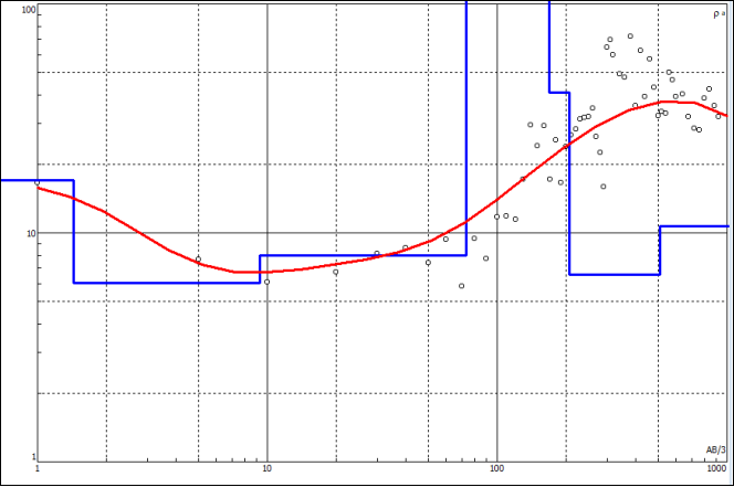
Figure 4. Modelled VES resistivity curve for station L1 (RMS error 10%).
Figure 5. Interpreted geoelectric section generated for VES station L1.
Lithologic attributes including true resistivity of the formation, depth and thickness or each resistivity layer are embedded in the ideal theoretical curve. During data processing, matching the acquired apparent resistivity values with the ideal field curve modifies the geoelectric properties of the rock layers and in many cases, additional geoelectric layers are added for a good representative match with reduced error.
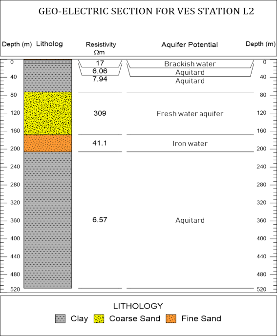
Vertical Electrical Sounding Line 2
Layer 1 extends from 0.0m at the surface to 1.44 m depth. The layer has a thickness of 1.44 m and a representative resistivity value of 17 Ωm. The layer has been interpreted as fine grained sand. The low resistivity values recorded for this interval suggest the presence of brackish water. The second geo-electric layer extends from 1.44 m to 9.27 m depth. The layer has a thickness of 7.83 m and a representative resistivity value of 6.06 Ωm. The layer has been interpreted as clay. Hence, this layer has no aquifer potential. Similarly, the third geo-electric layer extends from 9.27 m to 73.20 m depth. The layer has a thickness of 63.93 m and a representative resistivity value of 7.94 Ωm. The thick layer has been interpreted as clay with no aquifer potential. The fourth geo-electric layer extends from 73.20 m to 168 m depth. The layer has a thickness of 94.80 m and a representative resistivity value of 309 Ωm. The layer has been interpreted as fresh water coarse sand. Hence, this layer has an excellent aquifer potential and is of sufficient thickness. The fifth geo-electric layer extends from 168 m to 206 m depth. The layer has a thickness of 38.0 m and a representative resistivity value of 41.10 Ωm. The layer has been interpreted as a fine sandy unit bearing iron water. This layer has been interpreted as having fair aquifer potential. The sixth geo-electric layer extends from 206 m to 510 m depth. The layer has a thickness of 304 m and a representative resistivity value of 6.57 Ωm. This thick layer has been interpreted as a clayey unit with no aquiferous potential.
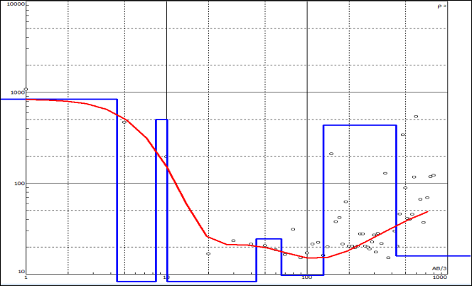
Figure 6. Modelled VES resistivity curve for station L2 (RMS error 18%).
Figure 7. Interpreted geoelectric section generated for VES station L2.
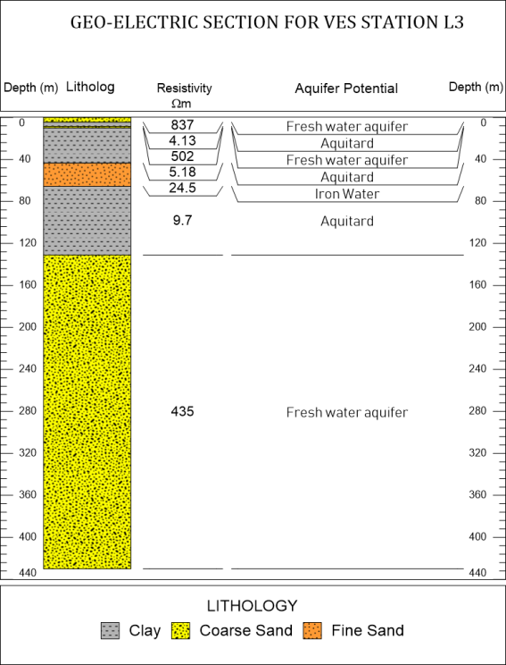
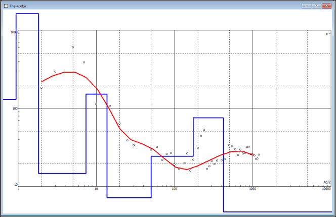
Figure 8. Modelled VES resistivity curve for station L3 (RMS error 18.5%).
Figure 9. Interpreted geoelectric section generated for VES station L3.
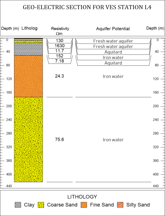
Figure 10. Modelled VES resistivity curve for station L4 (RMS error 14%).
Figure 11. Interpreted geoelectric section generated for VES station L4.
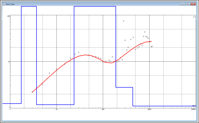
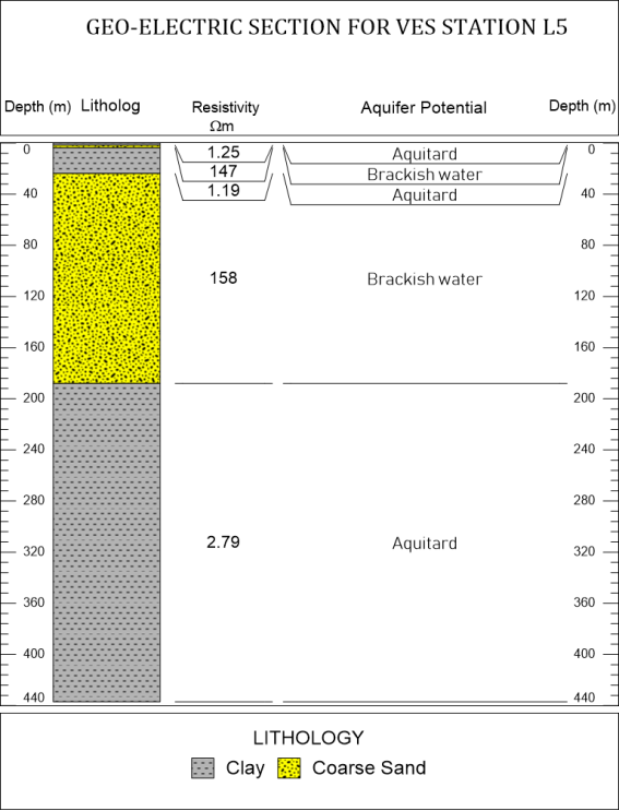
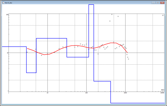
Figure 12. Modelled VES resistivity curve for station L5 (RMS error 12%).
Figure 13. Interpreted geoelectric section generated for VES station L5.
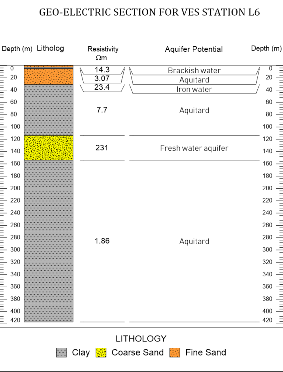
Figure 14. Modelled VES resistivity curve for station L6 (RMS error 16%).
Figure 15. Interpreted geoelectric section generated for VES station L6.
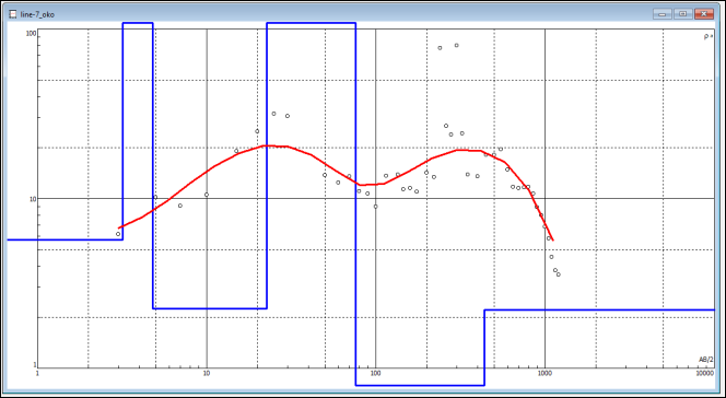
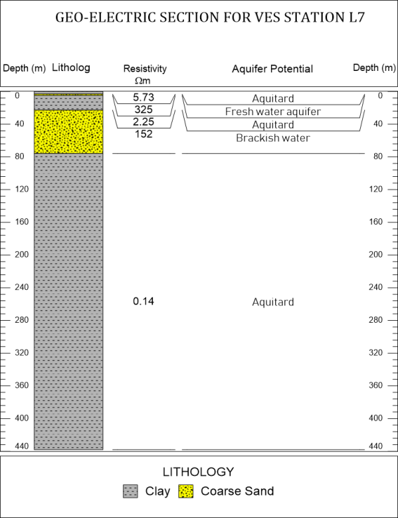
Figure 16. Modelled VES resistivity curve for station L7 (RMS error 15%).
Figure 17. Interpreted geoelectric section generated for VES station L7.
The interpreted resistivity values are based on the local geology of the Niger Delta and other regional guidelines (Keller and Frischknecht 1966; Daniels and Alberty 1966; Telford et al. 1990). Field apparent resistivity measurements were inverted to true resistivity values using IPI2win software. The true resistivity, number of geologic layers, the depth of occurrence and thickness of each geoelectric layer are the results obtained after a successful curve matching between acquired apparent resistivity values and the ideal theoretical curve. See Appendix B for Resistivity of some common rocks, soils and minerals utilized for this study.
Vertical Electrical Sounding Line 3
The field data acquired for VES survey line 3 along with the calculated apparent resistivity values indicates that Layer 1 extends from 0.0m at the surface to 4.46 m depth. The layer has a thickness of 4.46 m and a representative resistivity value of 837 Ωm. The layer has been interpreted as coarse grained sand. The high resistivity values recorded for this interval suggest the presence of fresh water sands with good aquifer potential. The second geo-electric layer extends from 4.46 m to 8.40 m depth. The layer has a thickness of 3.94 m and a representative resistivity value of 4.13 Ωm. The layer has been interpreted as clay. Hence, this layer has no aquifer potential. Layer 3 extends from 8.40m to 10.10 m depth. The layer has a thickness of 1.70 m and a representative resistivity value of 502 Ωm. The layer has been interpreted as coarse grained sand. The high resistivity values recorded for this interval suggest the presence of fresh water sands with excellent aquifer potential. The fourth geo-electric layer extends from 10.10 m to 43.50 m depth. The layer has a thickness of 33.40 m and a representative resistivity value of 5.18 Ωm. The thick layer has been interpreted as clay with no aquifer potential. The fifth geo-electric layer extends from 43.50 m to 65.60 m depth. The layer has a thickness of 22.10 m and a representative resistivity value of 24.50 Ωm. The layer has been interpreted as iron water rich fine sand. Hence, this layer has of fair aquifer potential. The sixth geo-electric layer extends from 65.60 m to 131 m depth. The layer has a thickness of 65.40 m and a representative resistivity value of 9.70 Ωm. The thick layer has been interpreted as clay with no aquifer potential. The seventh geo-electric layer extends from 131 m to 430 m depth. The layer has a thickness of 299 m and a representative resistivity value of 435 Ωm. The layer has been interpreted as fresh water coarse sand. Hence, this layer has an excellent aquifer potential and is of sufficient thickness.
Vertical Electrical Sounding Line 4
The interpreted VES survey line 4 along with the calculated apparent resistivity values depicts the area to be underlain by an eight geoelectric layers with layer 1 extending from 0.0m at the surface to 0.94 m depth. The layer has a thickness of 0.94 m and a representative resistivity value of 130 Ωm. The layer has been interpreted as silty sand. The resistivity values recorded for this interval suggest the presence of fresh water silty sands with good aquifer potential. The second geo-electric layer extends from 0.94 m to 1.83 m depth. The layer has a thickness of 0.89 m and a representative resistivity value of 1630 Ωm. The layer has been interpreted as coarse sand. Hence, this layer has excellent aquifer potential. Layer 3 extends from 1.83 m to 7.37 m depth. The layer has a thickness of 5.54 m and a representative resistivity value of 11.70 Ωm. The layer has been interpreted as clay with no aquifer potential. The fourth geo-electric layer extends from 7.37 m to 13.70 m depth. The layer has a thickness of 6.33 m and a representative resistivity value of 152 Ωm. The layer has been interpreted as coarse sand with iron water. The fifth geo-electric layer extends from 13.70 m to 50.20 m depth. The layer has a thickness of 36.50 m and a representative resistivity value of 7.18 Ωm. The thick layer has been interpreted as clay with no aquifer potential. The sixth geo-electric layer extends from 50.20 m to 173 m depth. The layer has a thickness of 122.80 m and a representative resistivity value of 24.30 Ωm. The thick layer has been interpreted as iron water rich fine sand with fair aquifer potential. The seventh geo-electric layer extends from 173 m to 422 m depth. The layer has a thickness of 249 m and a representative resistivity value of 75.60 Ωm. The layer has been interpreted as iron water coarse sand. Hence, this layer has a fair aquifer potential and is of sufficient thickness.
Vertical Electrical Sounding Line 5
VES line 5 depicts a 6-layer subsurface with layer 1 extending from ground surface to 1.73 m depth. The layer has a thickness of 1.73 m and a representative resistivity value of 1.25 Ωm. The layer has been interpreted as clay with no aquiferous potential. The second geo-electric layer extends from 1.73 m to 3.69 m depth. The layer has a thickness of 1.96 m and a representative resistivity value of 147 Ωm. The layer has been interpreted as brackish water coarse sand. Hence, this layer has poor aquifer potential. The third layer extends from 3.69 m to 23.80 m depth. The layer has a thickness of 20.11 m and a representative resistivity value of 1.19 Ωm. The layer has been interpreted as clay with no aquifer potential. The fourth geo-electric layer extends from 23.80 m to 188 m depth. The layer has a thickness of 164.20 m and a representative resistivity value of 158 Ωm. The layer has been interpreted as coarse sand saturated with brackish water. The fifth geo-electric layer extends from 188 m to 437 m depth. The layer has a thickness of 249 m and a representative resistivity value of 2.79 Ωm. This thick layer has been interpreted as clay with no aquifer potential.
Vertical Electrical Sounding Line 6
Layer 1 of VEs line 6 extends from 0.0m at the surface to 2.86 m depth. The layer has a thickness of 2.86 m and a representative resistivity value of 14.30 Ωm. The layer has been interpreted as fine sand saturated with brackish water. The second geo-electric layer extends from 2.86 m to 5.13 m depth. The layer has a thickness of 2.27 m and a representative resistivity value of 3.07 Ωm. This thick layer has been interpreted as clay with no aquifer potential. The third layer extends from 5.13 m to 31.10 m depth. The layer has a thickness of 25.97 m and a representative resistivity value of 23.40 Ωm. The layer has been interpreted as fine sand saturated with iron water. The fourth geo-electric layer extends from 31.10 m to 114 m depth. The layer has a thickness of 82.90 m and a representative resistivity value of 7.7 Ωm. This thick layer has been interpreted as clay with no aquifer potential. The fifth geo-electric layer extends from 114 m to 154 m depth. The layer has a thickness of 40 m and a representative resistivity value of 231 Ωm. This thick layer has been interpreted as coarse sand saturated with fresh water. This thick coarse sandy layer is sandwiched between two thick clayey layers, hence, the aquifer potential at this interval is excellent. The sixth geo-electric layer extends from 154 m to 417 m depth. The layer has a thickness of 263 m and a representative resistivity value of 1.86 Ωm. This thick layer has been interpreted as clay with no aquifer potential.
Vertical Electrical Sounding Line 7
Layer 1 extends from 0.0m at the surface to 3.19 m depth. The layer has a thickness of 3.19 m and a representative resistivity value of 5.73 Ωm. The layer has been interpreted as clay with no aquifer potential. The second geo-electric layer extends from 3.19 m to 4.80 m depth. The layer has a thickness of 161 m and a representative resistivity value of 325 Ωm. This layer has been interpreted as coarse sand saturated with fresh water. The third layer extends from 4.80 m to 22.70 m depth. The layer has a thickness of 17.90 m and a representative resistivity value of 2.25 Ωm. This layer has been interpreted as clay with no aquifer potential. The fourth geo-electric layer extends from 22.70 m to 75.90 m depth. The layer has a thickness of 53.20 m and a representative resistivity value of 152 Ωm. This thick layer has been interpreted as brackish water saturated coarse sand with poor aquifer potential. The fifth geo-electric layer extends from 75.90 m to 438 m depth. The layer has a thickness of 362.10 m and a representative resistivity value of 0.14 Ωm. This thick layer has been interpreted as clay with no aquifer potential.
4.2. Soil Profile of the Area
The soil profile for the area was interpreted based on the formation’s true resistivity values. Ideally, clayey soils have resistivity values while sandy soils have significantly higher resistivity values. The presence of a fluid phase in the soil significantly lowers the soil resistivity values. Hence, a sandy or clayey soil saturated with salt water will have a significantly lower resistivity value compared with fresh water saturated clays and sands. In this study, the lithologies identified included coarse sand, silty sand, fine sands and clay. Coarse sands and clays were the predominant lithologies identified in the area. VES lines L2, L5, L6 and L7 had thick clayey layers at the bottom of their profiles (
Figures 12, 15, 16, 17). Meanwhile VES points L1, L3, and L4 had thick sands towards the bottom of their profiles (
Figures 5, 7, 9, 11, 13, 15 and 17).
Figure 18. 3-D block model showing the various lithologic units interpreted from VES surveying.
Figure 19. Fence diagram showing the interconnectivity between lithologic units interpreted from VES surveying.
Figures 18–23 depicts the correlation of the subsurface lithologic layers and connectivity of the sand and clay layers across the survey window. The significant variations in the lithologies encountered between VES sounding points reflects the heterogenous nature of the soils in the area.
Figure 20. A profile along VES L4, L1 and L5 showing the interconnectivity between sandy units identified from VES survey.
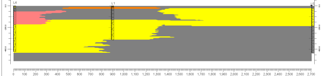
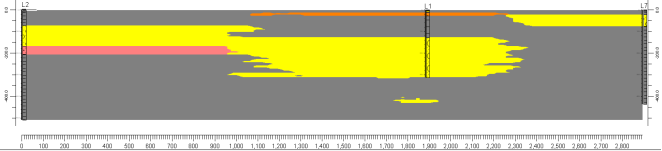
Figure 21. A profile along VES L2, L1 and L7 showing the interconnectivity between sandy units identified from VES survey.
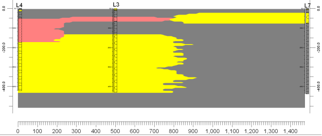
Figure 22. A profile along VES L4, L3 and L7 showing the interconnectivity between sandy units identified from VES survey.
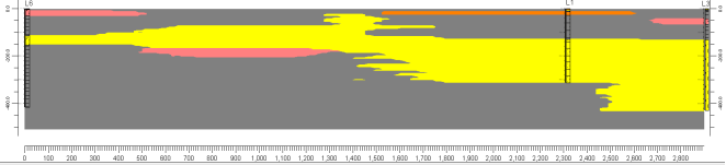
Figure 23. A profile along VES L6, L1 and L3 showing the interconnectivity between sandy units identified from VES survey.
4.3. Design of Abstraction Wells and Drilling Plan
The lithologic units identified in the area are predominantly clay and coarse sand. Fine sand and silty sand are not so predominant.
Figures 20 and 21 shows most part of the coarse sandy units are interconnected and lies within thick clayey units. Fresh water, iron rich water and brackish water are the fluid types encountered. Maximum investigation depth for groundwater in the area is 510 m. Deep groundwater (>110m) prospects with good quality can be obtained at VES points L2 (168 to 208m), L3 (131 to 430m) and L6 respectively (114 to 154m). VES points L1 and L4 have sands with sufficient thickness but can only provide water with iron content. No potable water was found at depths exceeding 5.0m depth at VES point L7. Thick clays with poor aquifer potentials (aquitard) predominates at shallow and deeper depths. VES point L3 provides the most suitable location to locate a deep borehole to obtain fresh water in the area (depth of borehole should extend to 430m and well screen should be installed from 131 to 430m. The thickness of the fresh water column in the confined aquifer is 299.0 m. The sand lies between 131 m and 430 m below ground surface. The thickness of the sand and the overlying thick clayey sealing layer makes VES point L3 the most viable prospect in the area for groundwater exploitation. The second most viable aquiferous drill target was found at VES point 6 at a depth from 114 to 154m. The thickness of this layer is 40 m. The freshwater coarse-grained sandy layer lies between two clayey layers with thicknesses of 82.80 m and 263 m at the top and bottom of the aquifer. The borehole depth to be drilled at this location should extend to 154m and well screen should be installed from 114 to 154m depth. The third drill target was found at VES point 2. Freshwater was encountered between 73.20 m and 168 m. The thickness of the aquiferous sand is 94.80 m. The freshwater coarse grained sandy aquifer is overlain by a 63.93 m thick clayey unit and underlain by a 38 m thick fine sandy layer. The underlying fine sandy layer is host to iron water. Hence, bentonite and cement can be used to seal off this layer prior to well development and production. The borehole depth to be drilled at this location should extend to 168m and well screen should be installed from 74m to 168m depth. Ves point 1 and VES point 4 represents drill targets for iron water. Aquiferous coarse sandy unit with iron water was encountered between 129 m and 314 m in VES point 1. The thickness of the aquifer is 185 m. Similarly, iron water was encountered between 50.2 m and 422 m in VES point 4. The thickness of the fine sand and coarse sand column containing iron water is 371.80 m. For production of iron water, significant treatment units have to be put in place prior to consumption.
5. Conclusion
The modelled true resistivity values after curve matching ranged between 0.14 Ohm.m and 1085 Ohm.m across all survey points. Total investigation depth ranged between 314.0m and 510.0m. True resistivity values between 0.14 Ohm.m and 7.94 Ohm.m were indicative of clayey formations. True resistivity values between 14.3 and 17 Ohm.m indicates Fine sandy formation with brackish water. True resistivity values between 23.40 Ohm.m and 41.10 Ohm m indicates the presence of Fine sands saturated with iron water. True resistivity values between 110 and 130 Ohm.m are indicative of Silty sands saturated with either fresh water or brackish water. True resistivity values between 139 and 158 Ohm.m suggests coarse sands saturated with iron water. True resistivity values between 231 and 1630 Ohm.m indicates the presence of fresh water sands. Hence, based on these resistivity values, fresh water was encountered only at L2 (borehole depth of 168m), L3 (borehole depth of 430m) and L6 VES locations (borehole depth of 154m).
The geology of the area is predominantly clayey which is followed by coarse grained sands. Silty sands and fine sands occupy a minor fraction of the total survey area. Thick aquiferous sands were found at various depths along VES points L1, L2, L3, L4 and L6 respectively. The aquiferous lithologies are mainly found in coarse sands and fine sands. Iron water is found in coarse sands at a depth interval from 129 m to 314 m at VES point L1. At VES point L2, fresh water coarse sands underlain by iron water saturated fine sands occurs at a depth interval from 73.20 m to 206 m depth. At VES point L3, fresh water saturated coarse sands were found at a depth interval from 131 m to 430 m depth. Borehole should be drilled to 430m depth and screened from 131m to the 430m at location L3. At VES point L4, fine sands overlying coarse grained sands were saturated with iron water from 50.20 m to 422 m depth. At VES point L6, fresh water saturated coarse grained sandy aquifer was found from 114 m to 154 m depth. Although VES point L2, L3 and L6 provides the most suitable prospective locations to cite a deep borehole to obtain fresh water in the area at depths 168m for L2, 430m for L3 and 154m for L6, lithologic modelling revealed that both coarse sands and fine sands are either juxtaposed or interfingered at the shallow, intermediate and deeper depths, hence, there is strong potential for iron water and fresh water inter-mixing as a result of exploitation.
All twenty (20) proposed boreholes to be drilled within Studied site’s plant area should not exceed a pumping rate of 3,500 liters per minute and each borehole should be located at distances exceeding 450m apart to prevent well interferences.
Although all twenty (20) boreholes have been proposed to be drilled within Studied site’s plant area, boreholes should be cited at varying depths between 150 and 450m. Five boreholes can be drilled to depths of 150m, 10 boreholes can be drilled to depths of 300m and 5 boreholes drilled to depths of 450m accordingly. This will greatly reduce stresses on the well field and also reduce the potential risk from saline intrusion.
A pumping schedule in which 10 to 14 boreholes can be active daily will also greatly reduce stresses on the well field and reduce the potential risk from saline intrusion.
Three monitoring boreholes (M1, M2 and M3) should be cited towards the East, West and Southern sections of the plant area for monitoring saline encroachment M1 is sited 1.5km away from L1. M2 is cited 1.50km away from L2 and M3 is located 2.40km away from L7. These boreholes are not producing boreholes but will be utilized solely for the purpose of salinity intrusion monitoring.
6. Recommendation
The study recommends the following;
1) Water treatment plants should be installed in order to help treat exploited iron water.
2) Pumping rates should be carefully monitored and not exceed 3,500 liters per minute. Pumping rate for L6 and L8 should be 2500. Pumping rate for L12 should be 2000 liters per minute, while pumping rate for all other boreholes should be kept at 3500 liters per minute flow rate This will reduce stress on the aquifer and the drawdown impact on the surrounding. Also, this will significantly prevent saline water encroachment.
a. Ground water modelling to be done for pump flow-100 m3/hr per pump (Total project water requirement is 7800 m3/hr)
b. How much water can be pumped keeping all boreholes 24 hours running
c. Distance between boreholes
d. All borehole location to be marked on Plot plan
e. Depth of all boreholes to be indicated
f. Length of screen for each borehole to be mentioned.
g. Location of pump inside each borehole to be mentioned
h. Location & depth of monitoring borehole to be mentioned on Plot plan.
3) All twenty (20) proposed boreholes to be drilled within Studied site’s plant area should be sited at distances exceeding 450m apart to prevent well interferences.
4) It may be required to consider using an additional geophysical surveying method that works on the principle of electromagnetism (EM) for confirmation prior to drilling. The EM surveys can be conducted using a hand-held EM device that gives results on the fly. This can be conducted on 4 proposed drill points. The points should be widely dispersed to account for heterogeneity of the soil formations.
5) Excessive groundwater exploitation from the area could lead to excessive settlement and subsidence of sections of the plant. Since the plant comprise several rigid skid systems, excessive pumping over a prolonged time could result in damage to structures within the plant. Five boreholes can be drilled to depths of 150m, 10 boreholes can be drilled to depths of 300m and 5 boreholes drilled to depths of 450m accordingly. This will greatly reduce stresses on the well field and also reduce the potential risk from saline intrusion.
6) Groundwater quality should be monitored regularly especially for the boreholes nearest to the coastline, due to the risks of saline intrusion arising from overpumping of the wellfield. When groundwater levels are lowered below Mean-sea level as a result of overpumping, it could trigger a reversal in groundwater flow direction, thereby causing saline intrusion into the well field. (Groundwater samples can be collected monthly for salinity and conductivity test, or a data logger with TDS and chloride content recorder can be installed permanently in the borehole after casing. Results from the data logger can be acquired remotely based on preset protocols prior to installation).
7) Lastly, it is recommended that complimentary Downhole Logs comprising Resistivity (SP Short and Long Normal), and Gamma Ray must be run prior to casing to determine screening horizons and to enhance delivery of groundwater of suitable quality. (Logging has to be done for all Boreholes prior to casing).
Abbreviations
VES | Vertical Electrical Sounding |
HRP | Horizontal Resistivity Profiling |
L | Location |
SP | Self-potential |
Author Contributions
Tamunoene Kingdom Simeon Abam: Conceptualization, Formal Analysis, Funding acquisition, Methodology, Project administration, Supervision, Validation
Paul Mokam Mogaba: Project administration, Software, Validation, Visualization
Fidelis Ankwo Abija: Data curation, Validation, Visualization, Writing – original draft, Writing – review & editing
Conflicts of Interest
The authors declare no conflicts of interest.
References
| [1] |
Than, N. N., Thunyawatcharakul, P., Ngu, N. H. and Chotpantarat, S. (2022). Global review Global review of groundwater potential models in the last decade: Parameters, model techniques, and validation. Journal of Hydrology, Volume 614, Part A, November 2022, 128501.
|
| [2] |
Abija, F. A., Abam, T. K. S., Teme, S. C. and Eze, C. L. (2011). Relative Sea Level Rise, Coastline Variability and Coastal Erosion in the Niger Delta, Nigeria: Implications for Climate Change Adaptation and Coastal Zone Management. J. Earth Science and Climate Change vol., 11:9, pp. 1–10. FOR code: 240504.
|
| [3] |
Abija, F. A., Harry, I. M. and Udom, G. J. (2020). Sources of Salinization and Investigation of Salt Water Intrusion into Coastal Aquifers in Parts of the Niger Delta, Nigeria. Journal Hydrogeology and Hydrologic Engineering, vol., 9:4, pp. 1–8.
|
| [4] |
Baydon-Ghyben, W. (1889). Nota in verban met de voorgenomen putboring nabij Amsterdam., Koninlyk Instituut Ingennieurs Tidjchrift (The Hauge) 1888 – 1889, pp. 8–22.
|
| [5] |
Herzberg, A. (1901). “Die Wasserversorgung einiger Nordseebader”. Journal Gasbeleuchtung und Wasserversorgung (Munich), 44(1901), 815–19, 842-44.
|
| [6] |
Abam, T. K. S. and Nwankwoala, H. O. (2020) Hydrogeology of Eastern Niger Delta: a Review. Journal of Water Resource and Protection, 2020, 12, 741-777.
|
| [7] |
Ngah, S. A. and Nwankwoala, H. O. (2013) Assessment of Static Water Level Dynamics in Parts of the Eastern Niger Delta. The International Journal of Engineering and Science, 2, 136-141.
|
| [8] |
Ngah S. A (2009) Deep Aquifer Systems of Eastern Niger Delta: Their Hydrogeological Properties, Groundwater Chemistry and Vulnerability to Degradation, PhD Thesis, Rivers State University, Port-Harcourt, Nigeria.
|
| [9] |
Abam, T. K. S. (2001). Regional hydroiogical research perspectives in the Niger Delta. Hydroiogical Sciences- Hydroiogical Sciences-,)'ouriwl-des Sciences Hydrologiques, 46(1), pp. 13-32.
|
| [10] |
Edwards, K. A., Classen, G. A. and Schroten, E. H. J. (1983) The Water Resource in Tropical Africa and Its Exploitation. E-Book Series. ILCA Publications, 103 p.
|
| [11] |
Abija, F. A., Essien, N. U., Abam, T. K. S and Ifedotun, A. I. (2019). Assessment of Aquifer Hydraulic Properties, Groundwater Potential and Vulnerability Integrating Geoelectric Methods with SRTM -DEM and LANDSAT -7 ETM lineament Analysis in Parts of Cross River State, Nigeria. London Journal of Research in Science: Natural and Formal, Volume 19 | Issue 7 | Compilation 1.0, pp. 35–51.
|
| [12] |
Wikipedia.
https://en.wikipedia.org/wiki/Water_potential
|
| [13] |
Fetter CW (1988) Applied hydrogeology, 2nd edn. CBS Publishers, New Delhi.
|
| [14] |
Kebede, S. (2013). Groundwater Potential, Recharge, Water Balance: Vital Numbers. In: Groundwater in Ethiopia. Springer Hydrogeology. Springer, Berlin, Heidelberg.
|
| [15] |
Ugbaja, A. N., William, G. A. and Ugbaja, A. A. (2021). Evaluation of groundwater potential using aquifer characteristics on parts of boki area, south – eastern nigeria. Global journal of geological sciences vol. 19, 2021: 93-104.
|
| [16] |
Zhang, Z. Zhang, S., Li, M. Zhang, Y., Chen, M., Zhang, Q. Dai, Z. and Liu, J. (2023). Groundwater Potential Assessment in Gannan Region, China, Using the Soil and Water Assessment Tool Model and GIS-Based Analytical Hierarchical Process. Remote Sens., 15(15), 3873.
|
| [17] |
Yohana, A. R., Makoba, E. E., Mussa, K. R., Mjemah, I. C. (2023). Evaluation of Groundwater Potential Using Aquifer Characteristics in Urambo District, Tabora Region, Tanzania. Earth 2023, 4(4), 776-805.
|
| [18] |
Ehirim, C. N. and Nwankwo, C. (2016) Quality Assessment and Evaluation of Groundwater Potentials in Parts of Buruku and Gboko Local Government Area Councils in Benue State. International Journal of Geosciences, 7, 1064-1073.
|
| [19] |
Aizebeokhai, A. P., Oyeyemi, K. D. and Joel, E. S. (2016). Groundwater potential assessment in a sedimentary terrain, southwestern Nigeria. Arab J Geosci (2016) 9:496 pp. 2–15.
|
| [20] |
Alabi, A. A., Popoola, O. I., Olurin, O. T. et al. Assessment of groundwater potential and quality using geophysical and physicochemical methods in the basement terrain of Southwestern, Nigeria. Environ Earth Sci 79, 364 (2020).
|
| [21] |
Ekwok, S. E., Akpan, A. E., Kudamnya, E. A. and Ebong, E. D. (2020). Assessment of groundwater potential using geophysical data: a case study in parts of Cross River State, south eastern Nigeria. Applied Water Science (2020) 10: 144.
|
| [22] |
Arafa, S. A. S., Hamed, H., Nayef, A., Sabet, H. S., AbuBakr, M. M., and Mebed, M. E. (2023). Assessment of groundwater aquifer using geophysical and remote sensing data on the area of Central Sinai, Egypt. Scientifc Reports | (2023) 13:18245, pp. 1–18.
|
| [23] |
Ubaidullah, A., Francis, A. A. and Francis, W. K. (2021). Assessment of groundwater potential using vertical electric sounding technique at Faculty of Medicine and Engineering, Federal University Dutsin-ma Katsina State, Nigeria. Global Journal of Earth and Environmental Science Volume 6(4), pages 98-105.
|
| [24] |
Li, K., Yan, J., Li, F., Lu, K., Yu, Y., Yulin Li, Y. Zhang, L., Wang, P. Li, Z., Yang, Y. and Wang, J. (2014). Non invasive geophysical methods for monitoring the shallow aquifer based on time lapse electrical resistivity tomography, magnetic resonance sounding, and spontaneous potential methods. Scientifc Reports | (2024) 14:7320, pp. 1-12.
|
| [25] |
Raji, W. O. and Abdulkadir, K. A. (2023). Evaluation of groundwater potential of bedrock aquifers in Geological Sheet 223 Ilorin, Nigeria, using geo electric sounding. Applied Water Science (2020) 10:220 pp. 1-12.
|
| [26] |
Duguma, T. A. and Duguma, G. A. (2022). Assessment of Groundwater Potential Zones of Upper Blue Nile River Basin Using Multi-Influencing Factors under GIS and RS Environment: A Case Study on Guder Watersheds, Abay Basin, Oromia Region, Ethiopia. Geofluids Volume 2022, Article ID 1172039, pp 1–26.
|
| [27] |
Boitt, M., Khayasi, P. and Wambua, C. (2023) Assessment of Groundwater Potential and Prediction of the Potential Trend up to 2042 Using GIS-Based Model and Remote Sensing Techniques for Kiambu County. International Journal of Geosciences, 14, 1036-1063.
|
| [28] |
Tamesgen, Y, Atlabachew, A. and Jothimani, M. (2023). Groundwater potential assessment in the Blue Nile River catchment, Ethiopia, using geospatial and multi-criteria decision-making techniques. Heliyon 9 (2023) e17616 pp. 1–21.
|
| [29] |
Opoku, P. A.; Shu, L.; Amoako-Nimako, G. K. (2024). Assessment of Groundwater Potential Zones by Integrating Hydrogeological Data, Geographic Information Systems, Remote Sensing, and Analytical Hierarchical Process Techniques in the Jinan Karst Spring Basin of China. Water 2024, 16, 566.
|
| [30] |
Amajor, L. C. (1991) Aquifers in the Benin Formation (Miocene-Recent) Eastern Niger Delta, Nigeria: Lithostraigraphy, Hydraulics and Water Quality. Environmental Geology and Water Sciences, 17, 85-101.
https://doi.org/10.1007/BF01701565
|
| [31] |
Etu-Efeotor, J. O. and Odigi, M. I. (1983). Water Supply Problems in the Niger Delta. J. of Mining and Geology, vol. 20 (1&2), pp. 183–193.
|
| [32] |
Akpokodje, E. G., Etu-Efeotor, J. O. and Mbeledogu, I. U. (1996) A Study of Environmental Effects of Deep Subsurface Injection of Drilling Waste on Water Re- sources of the Niger Delta. CORDEC, University of Port Harcourt, Port Harcourt.
|
| [33] |
Akpoborie, I. A. (2011) Aspects of the Hydrology of the Western Niger Delta Wetlands: Groundwater Conditions in the Neogene (Recent) Deposits of the Ndokwa Area. Proceedings of the Environmental Management Conference, Federal University of Agriculture, Abeokuta, 13 p.
|
Cite This Article
-
APA Style
Abam, T. K. S., Mogaba, P. M., Abija, F. A. (2024). Assessment of Groundwater Potential in Parts of the Coastal Niger Delta, Nigeria: Implications for Well Design. Journal of Water Resources and Ocean Science, 13(6), 136-157. https://doi.org/10.11648/j.wros.20241306.11
 Copy
|
Copy
|
 Download
ACS Style
Abam, T. K. S.; Mogaba, P. M.; Abija, F. A. Assessment of Groundwater Potential in Parts of the Coastal Niger Delta, Nigeria: Implications for Well Design. J. Water Resour. Ocean Sci. 2024, 13(6), 136-157. doi: 10.11648/j.wros.20241306.11
Copy
|
Download
AMA Style
Abam TKS, Mogaba PM, Abija FA. Assessment of Groundwater Potential in Parts of the Coastal Niger Delta, Nigeria: Implications for Well Design. J Water Resour Ocean Sci. 2024;13(6):136-157. doi: 10.11648/j.wros.20241306.11
Copy
|
Download
-
@article{10.11648/j.wros.20241306.11,
  author = {Tamunoene Kingdom Simeon Abam and Paul Mokam Mogaba and Fidelis Ankwo Abija},
  title = {Assessment of Groundwater Potential in Parts of the Coastal Niger Delta, Nigeria: Implications for Well Design},
  journal = {Journal of Water Resources and Ocean Science},
  volume = {13},
  number = {6},
  pages = {136-157},
  doi = {10.11648/j.wros.20241306.11},
  url = {https://doi.org/10.11648/j.wros.20241306.11},
  eprint = {https://article.sciencepublishinggroup.com/pdf/10.11648.j.wros.20241306.11},
  abstract = {The location, design, drilling and completion of wells for potable groundwater abstraction require exploration and mapping of groundwater potential zones within the geologic framework of any region. In this study, field data acquisition involved seven vertical electrical sounding and three horizontal resistivity profiling (HRP) carried out. Field data were interpreted using IPI2win 1-D software while subsurface lithologic layering and correlation was realized in rockworks v 22. Modelled true geolectric sections after curve matching revealed the study area to be underlain predominantly by clayey lithologic units followed by coarse grained sands with silty sands and fine sands in minor fraction. Total investigation depth range between 314.0m and 510.0m and fresh water was found to occur at a depth of 168m in VES L2, 430m in VES L3 and 154m in VES L6 locations. Iron water was found in some coarse sands at a depth interval of 129 m to 314 m at VES L1 while fresh water in coarse sands underlain by iron water saturated fine sands occurs at a depth interval of 73.20 m to 206 m at VES L2. At VES L3, fresh water saturated coarse sands were found at a depth interval of 131 m to 430m. Boreholes should be drilled to 430m and screened from 131m to 430m at L3. At VES L4, fine sands overlying coarse grained sands were saturated with iron water from 50.20 m to 422m. At VES L6, fresh water saturated coarse grained sandy aquifer was found from 114 m to 154m. Although VES L2, L3 and L6 provides the most suitable prospective locations for fresh water in the area at depths of 168m for L2, 430m for L3 and 154m for L6, lithologic modelling revealed that both coarse sands and fine sands are either juxtaposed or interfingered at the shallow, intermediate and deeper depths, hence, there is strong potential for iron water and fresh water inter-mixing during pumping. All twenty proposed boreholes are recommended not to be pumped at rates exceeding 3,500 l/min. Boreholes should be 450m apart to prevent well interferences and pumping schedule of 10 to 14 boreholes daily will greatly reduce stresses on the well field as well as potential risk from saline intrusion. Three saline water encroachment monitoring boreholes should be sited at 1.5km from L1 and L2 and 2.4km from L7 respectively at the East, West and Southern sections of the plant area.},
 year = {2024}
}
Copy
|
Download
-
TY  - JOUR
T1  - Assessment of Groundwater Potential in Parts of the Coastal Niger Delta, Nigeria: Implications for Well Design
AU  - Tamunoene Kingdom Simeon Abam
AU  - Paul Mokam Mogaba
AU  - Fidelis Ankwo Abija
Y1  - 2024/12/30
PY  - 2024
N1  - https://doi.org/10.11648/j.wros.20241306.11
DO  - 10.11648/j.wros.20241306.11
T2  - Journal of Water Resources and Ocean Science
JF  - Journal of Water Resources and Ocean Science
JO  - Journal of Water Resources and Ocean Science
SP  - 136
EP  - 157
PB  - Science Publishing Group
SN  - 2328-7993
UR  - https://doi.org/10.11648/j.wros.20241306.11
AB  - The location, design, drilling and completion of wells for potable groundwater abstraction require exploration and mapping of groundwater potential zones within the geologic framework of any region. In this study, field data acquisition involved seven vertical electrical sounding and three horizontal resistivity profiling (HRP) carried out. Field data were interpreted using IPI2win 1-D software while subsurface lithologic layering and correlation was realized in rockworks v 22. Modelled true geolectric sections after curve matching revealed the study area to be underlain predominantly by clayey lithologic units followed by coarse grained sands with silty sands and fine sands in minor fraction. Total investigation depth range between 314.0m and 510.0m and fresh water was found to occur at a depth of 168m in VES L2, 430m in VES L3 and 154m in VES L6 locations. Iron water was found in some coarse sands at a depth interval of 129 m to 314 m at VES L1 while fresh water in coarse sands underlain by iron water saturated fine sands occurs at a depth interval of 73.20 m to 206 m at VES L2. At VES L3, fresh water saturated coarse sands were found at a depth interval of 131 m to 430m. Boreholes should be drilled to 430m and screened from 131m to 430m at L3. At VES L4, fine sands overlying coarse grained sands were saturated with iron water from 50.20 m to 422m. At VES L6, fresh water saturated coarse grained sandy aquifer was found from 114 m to 154m. Although VES L2, L3 and L6 provides the most suitable prospective locations for fresh water in the area at depths of 168m for L2, 430m for L3 and 154m for L6, lithologic modelling revealed that both coarse sands and fine sands are either juxtaposed or interfingered at the shallow, intermediate and deeper depths, hence, there is strong potential for iron water and fresh water inter-mixing during pumping. All twenty proposed boreholes are recommended not to be pumped at rates exceeding 3,500 l/min. Boreholes should be 450m apart to prevent well interferences and pumping schedule of 10 to 14 boreholes daily will greatly reduce stresses on the well field as well as potential risk from saline intrusion. Three saline water encroachment monitoring boreholes should be sited at 1.5km from L1 and L2 and 2.4km from L7 respectively at the East, West and Southern sections of the plant area.
VL  - 13
IS  - 6
ER  -
Copy
|
Download