The Maximum Attainable Flow and Minimal Cost Problem in a Network

Amanuel Belachew Beyi; Temesgen Alemu Godana

doi:doi:10.11648/j.ajmcm.20240902.11

Review Article |

| Peer-Reviewed

The Maximum Attainable Flow and Minimal Cost Problem in a Network

Amanuel Belachew Beyi, Temesgen Alemu Godana^*

Published in American Journal of Mathematical and Computer Modelling (Volume 9, Issue 2)

Received: 31 March 2024 Accepted: 6 May 2024 Published: 17 May 2024

Views: Downloads:

Download PDF

Share This Article

Twitter
Linked In
Facebook

Abstract

This paper, presents an efficient algorithm that solves such a large class of optimization problems. Ford-Fulkerson determines the maximum flow in a network by iteratively augmenting flow paths until no further improvement is possible. On the other hand, Dijkstra's algorithm excels in finding the shortest path in a weighted graph, making it suitable for minimizing costs in network traversal. However, this paper simultaneously optimizes both objectives (flow and cost) dependently in unique iterations by considering all constraints and objectives holistically. The aim of this work is to develop efficient algorithms that can handle complex optimization problems in transportation, network design, and other fields, ultimately improving resource utilization and minimizing costs as its crucial for enhancing decision-making processes, improving efficiency in resource utilization, and achieving cost savings in diverse applications ranging from transportation networks to production planning. This paper deals about formulating the linear programming for the optimizations problems and finding the maximum amount of flow that can be sent from a source node to a sink node while minimizing the total cost of sending that flow by using simplex method (Two phase method). Through computational experiments and case studies, everybody demonstrate the effectiveness and efficiency of the proposed approach in solving real-world network flow problems. Our method yields efficient algorithms with in smallest numbers of iterations and time that enable the optimal allocation of resources within networks, achieving both maximum flow and minimum cost simultaneously.

Published in	American Journal of Mathematical and Computer Modelling (Volume 9, Issue 2)
DOI	10.11648/j.ajmcm.20240902.11
Page(s)	22-37
Creative Commons	This is an Open Access article, distributed under the terms of the Creative Commons Attribution 4.0 International License (http://creativecommons.org/licenses/by/4.0/), which permits unrestricted use, distribution and reproduction in any medium or format, provided the original work is properly cited.
Copyright	Copyright © The Author(s), 2024. Published by Science Publishing Group

Keywords

Maximum Flow, Minimum Cost, Linear Programming, Network Flow Optimization, Two Phase Method

1. Introduction

Mathematical optimizations are applicable in almost all real world life problems such as diet problem, inventory problem, transportation planning, network design, and supply chain. Network optimization models have been most exciting developments in operation research in recent years

[1-3]

. They are widely used in optimization problems which have countless practical applications in various fields including commodity transportation, telecommunication systems, network design, resource planning, scheduling, railroad and highway traffic planning, electrical power distribution, project planning, facilities location, resource management, and financial planning and much more

[4, 5]

. The fundamental question in network optimization is how to efficiently transport some entity (commodity, product, electrical power, vehicles, water etc.) from one point to another in a network while considering the amount of budget

[6, 7]

Network optimization is a special type of linear programming model. Some special types of network optimization models include: transportation problems, assignment problems, shortest path problems, minimum spanning tree problems, maximum flow problems, Chinese postman problem, knapsack problem and minimum cost flow problems

[8, 9]

. Solving it efficiently requires a deep understanding of graph theory, optimization techniques, and algorithmic design. The textbook

[10-12]

is an exhaustive reference on the subject. Maximum flow problem

[13-15]

, minimum cost problem (MCF) is a central problem in network flows.

Dantzig first proposed the idea of the Minimum Cost Flow Problem and created the first method to solve it in 1951. Conversely, T. Harris and F. Ross formulated the problem of the maximum flow discovery in a universal manner. For this problem, L. Ford and D. Fulkerson

[16, 13, 17]

created the well-known "augmented path" algorithm. The Ford-Fulkerson algorithm exists in many variants

[13, 18]

. One of these is the shortest path algorithm, which was put forth by J. Edmonds and R. Karp in 1972 and allows one to select the shortest supplementary path (assuming unit length for each arc) from the source to the sink at each step in the residual network

[19]

The paper on the minimum-cost flow problem and its applications in networks was published by Nguyen Viet Anh. This work focused on the least cost flow problem, where a constant cost function was not required. Both convex and differentiable functions are possible. For the maximum flow problem, they have expanded and changed the Ford-Fulkerson algorithm

[20, 21]

In the context of Maximum flow minimum cost problems, the cost associated with sending flow through network edges may represent transportation expenses, communication delays, or usage fees, among other considerations. Understanding and appropriately defining these costs is essential for accurately modeling the problem and devising efficient optimization strategies that balance flow maximization with cost minimization, taking into account the multifaceted nature of cost in network operations. Jewell

[24]

, Busaker and Gowen

[22, 23]

independently developed the successive shortest path algorithm

[24, 25]

. These researchers showed how to solve the MCF as a sequence of shortest path problems with arbitrary arc lengths. Edmonds and Karp

[3]

independently observed that if the computations use vertex potentials, it is possible to implement these algorithms so that the shortest path problems have non-negative arc lengths.

However, to the best of our knowledge, no one has proposed the work on solving maximum flow minimum cost simultaneously (dependently) using linear programming. In this work for the given weighted and directed graphs by which capacity and cost associated with them we formulate it as a linear programming and solve it using two phase method. The primary objective of this study attempted to achieve an optimal solution that balances the trade-offs between flow maximization and cost minimization, leading to efficient and cost-effective operation of the underlying network or system simultaneously. Obviously, the aim of this paper is to maximize flows and to minimize cost for a certain weighted digraphs in the network.

The last part of this paper, tried to demonstrate this algorithm and show some their applications in a real network.

2. Preliminaries

For given directed network, i.e. a directed graph with non-negative capacities on its edges, and two distinguished vertices source - s and sink – t, the maximum flow problem tries to find out a maximum flow from s to t in which each arc (i, j) has a maximum allowed capacity of u_ij.

In expanding our modeling approach, we introduce additional parameters, c_ij and u_ij, associated with each arc (i, j). Here, c_ij represents the cost of sending a unit of flow along the arc (i, j), while u_ij denotes the capacity constraint on that arc, indicating the maximum flow that can traverse it

[16, 23].

These parameters add depth to our understanding of the network by capturing the specific costs and capacities associated with individual connections. By incorporating these parameters into the problem formulation, this paper develop more nuanced optimization strategies that consider both the cost-effectiveness of flow distribution and the physical limitations imposed by the network topology.

Real networks can be modeled as a directed graph G= (V, A), where V is the set of n vertices (|V| = n) and A is the set of directed arcs. Each vertex symbolizes a location or node where resources originate, terminate, or transit, with associated attributes like production, demand, or capacity, crucial for optimizing flow distribution and minimizing costs. These vertices serve as key elements in formulating constraints and objectives governing flow dynamics, facilitating efficient resource allocation and logistics planning within the network

[8, 17]

. The source vertex denotes the origin of the flow, while the sink vertex represents its destination. Intermediate vertices facilitate the flow transfer between the source and sink, and their connectivity via edges dictates the flow paths.

Additionally, each vertex may have associated parameters such as production or consumption rates, capacities, and costs, which influence the flow optimization process

[5, 11, 14]

. By collectively considering the vertices and their interconnections, a comprehensive representation of the network topology and its flow characteristics can be established, enabling the application of optimization techniques such as linear programming to solve for maximum flow with minimum cost

[4, 7]

A network is a collection of points, called vertices (nodes), and a collection of lines, Called edges (arcs), connecting these points. Network topology is only one part of the graph. A network can be visualized by drawing the nodes as circles and the arcs as lines between them

[3, 8]

In operation of networks routing refers to the process of determining the path that data, information, or other entities take as they traverse through a network from a source to a destination

[7]

. Next section, present the formulation, algorithm and simultaneous solution methods of min-cost and maximum flow problem that plays an important role in network routing algorithm.

3. LP- Problem Formulation

Let G = (V, A) be a directed network with a cost c_ijand a capacity u_ijassociated with every arc (i, j) ∈A. For any i-j dipath, let P⁺ = set of all forward arcs on P (i,j) and P^- = set of all backward arcs on P (j,i) that means for vertex i in G, we define the Set of nodes before i - NB(i) and Set of nodes after i - NA(i) as follows. Let G = (V, A) be a digraph and iV. Then,

i. NB(i) = k V: (k, i)  A (Read as “Set of nodes before i ”)

ii. NA(i) = j V: (i, j)  A (Read as “Set of nodes After i ”)

Notation: For any i-j dipath, P⁺ = set of all forward arcs on P and P^- = set of all backward arcs on P is defined as:

P⁺(i)={j∈X|(i,j)∈A}(1)

P^-(i)={j∈X|(j,i)∈A}

Remark: (Flow Augmented Path (FAP))

A path P from s to t is an FAP if and only if the following conditions hold:

(i)

x_ij<u_ij,forall(i,j)P⁺(2)

(ii) x_ij > 0, for all (i, j)  P^-.

To determine a maximum flow through a FAP P, let

₁=min{u_ij–x_ij:(i,j)P⁺};and

₂=min{x_ij:(i,j)P^-}(3)

Then,  = min{₁, ₂}, called residual capacity of P, is the maximum flow that can be sent through P. Hence, the new flow in the network will be

x_ij

= \{\begin{matrix} x_{ij} + ∆, (i, j) \in P^{+} \\ x_{ij} - ∆, (i, j) \in P^{-} \\ x_{ij}, Otherwise \end{matrix}

(4)

is called flow augmentation

Note: In networks aiming to solve the maximum flow and minimum cost problem, the network cannot be in its optimal solution.

Note that: Flow augmentation increases the value of a flow by  and the new flow is feasible since whatever comes into a node still goes out of the node.

There are three types of nodes in a minimum cost flow problem: supply node, demand node, and transshipment node. A supply node is defined as a node where the flow out of the node exceeds the flow into the node. Similarly, a demand node is where the flow into the node exceeds the flow out of the node. A transshipment node (intermediate node) is where the flow into the node equals the flow out of the node. For example, a distribution network would include the sources of the goods being distributed (supply nodes), the customers (demand nodes) and intermediate storage facilities (transshipment nodes)

[7]

Download: Download full-size image

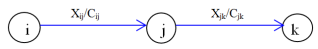
Figure 1. Source and sink digraphs.

Write (i, j) ∈A to say that there is an arc between nodes i ∈ V and j∈ V. In a directed network, the arc (i, j) is regarded as extending from node i to node j typically, a directed network model involves a flow or transportation of something along the arcs, in the specified directions. In an undirected network, the arc (i, j) just represents a connection between nodes i and j an undirected network model may allow flows in either direction along an arc, or may not involve explicit flows at all. Solving the maximum flow minimum cost problem simultaneously using linear programming involves formulating a linear program with decision variables representing the flow on each arc and the cost associated with each flow

[19]

Now, let us discuss methods to formulate linear programming for the directed and weighted graphs as optimization problems by which cost, capacity and flow are associated with them. Let’s consider a directed graph with nodes s (source) and t (sink), and several intermediate nodes and let us define structure of linear programming in case of graphs

[22, 23]

. Each edge has a capacity and a cost associated with sending flow through it. The following are definition of the structure of LP for solving maximum flow and minimum cost dependently:

1. Decision Variables: These represent the flow of goods, information, or any other entity through the arcs of the network. Typically, for each arcs (i, j) in the digraph, a decision variable x_ij is defined to denote the flow from vertex i to vertex j which are always non –negative (f_ij ≥ 0). That means, f_ij represent the flow on edge ij, where i and j are nodes and c_ij represent the cost of sending flow through edge ij. On each arc, there are 2 numbers indicating flow / cost respectively (fij /cij) where c_ij the cost per unit of flow on the edge c_ij i.e from node i to j.

2. Objective Function: The objective function aims to minimize the total cost of the flow while maximizing the flow through the network. It is typically represented as a linear combination of flow variables and their associated costs. For example, if c_ij represents the cost per unit of flow on edge (i, j), and f_ij represents the flow on that edge, then the objective function could be something like:

Min \sum_{(i, j) \in A} c_{ij ∙} f_{ij}

(5)

3. Constraints: The constraints ensure that the flow meets the requirements of the network and obeys the conservation of flow principle. They typically include:

i. Flow Conservation Constraints: For each Intermediate vertex i (except the source and sink), the total flow into the vertex must equal the total flow out of the vertex. Mathematically, it is expressed as;

\sum_{(i, j) \in A \ {s, t}} f_{ij -} \sum_{(j, k) \in A \ {s, t}} f_{jk} = 0

(6)

and Non-negative flow f_ij≥ 0.

b). capacity Constraints: These restrict the flow on each arc to be within its capacity limits i.e every flow on each arc should be less than or equals to the capacity possibly equals to zero. Mathematically, it is expressed as;

0≤f_ij≤u_ij(7)

c). Source and Sink Constraints: These specify that the total flow into the sink (demand) and out of the source (supply) must meet certain requirements. Mathematically, expressed as;

\sum_{(s, i) \in A} f_{sj -} \sum_{(j, s) \in A} f_{js} = Supply

(8)

\sum_{(i, t) \in A} f_{it -} \sum_{(t, i) \in A} f_{ti} = Demand

Where, s represents the source vertex and t represents the sink vertex.

Additional Constraints: To ensure that the flow out of the source equals the flow into the sink, set

\sum_{(s, v) \in A} f_{sv} = \sum_{(v, t) \in A} f_{vt}

(9)

Those using this all information use a linear programming solver two phase method (because constraints contains ≤ and =) so, solve it needs to convert in Perfect standard form (PSF) by introducing slack and artificial variables to solve the formulated linear program. This will provide the optimal flow values that minimize the total cost while satisfying the capacity and flow conservation constraints.

Let f_ijrepresent the flow along edge (i, j), c_ijrepresent the cost per unit flow along edge (i, j), and uij represent the capacity of edge (i, j). Linear programming formulated form of the problems arranged as follows. Objective function: Minimize the total cost equation (5):

Min \sum_{(i, j) \in A} c_{ij ∙} f_{ij}

Subject to: Capacity constraints: f_ij ≤ u_ij for all (i, j) in the digraph.

Conservation of flow: For each node i in the digraph (except the source and sink):

\sum_{(j, i) \in A} f_{ji -} \sum_{(i, j) \in A} f_{ij} = 0

Flow conservation at the source and sink nodes:

\sum_{(s, i) \in A} f_{sj -} \sum_{(j, s) \in A} f_{js} = Max flow

(10)

\sum_{(i, t) \in A} f_{it -} \sum_{(t, i) \in A} f_{ti} = - \max flow

Non-negativity constraints: f_ij ≥ 0 for all (i, j) in the digraph.

Note: Both Minimum cost and maximum flow problems are typically formulated on a directed graph where nodes represent locations and edges represent connections between them.

Example 1: Formulate linear programming problems for the given digraphs in figure 1 below with cost and capacity associated with it from source to sink node.

Download: Download full-size image

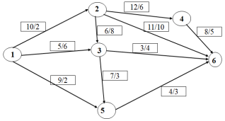
Figure 2. Examples of LP formulations of the networks.

Solution: There are six nodes: Source (1), Sink (6), Intermediate (2, 3 4, 5). There are ten arcs with their respective capacities and costs. For instance, considering the above figure we have the following:

(1, 2): Capacity = 10, Cost per unit flow = 2

(1, 3): Capacity = 5, Cost per unit flow = 6

(1, 5): Capacity = 9, Cost per unit flow = 2

(2, 3): Capacity = 6, Cost per unit flow = 8

(3, 5): Capacity = 7, Cost per unit flow = 3 etc..

Objective function: Minimize the total cost:

Minimize2f₁₂+6f₁₃+2f₁₅+8f₂₃+3f₃₅+6f₂₄+10f₂₆+4f₃₆+3f₅₆+5f₄₆

Subject to: Capacity constraints:

f₁₂≤10

f₁₃≤5

f₁₅≤9

f₂₃≤6

f₃₅≤7

f₂₄≤12

f₂₆≤11

f₃₆≤3

f₅₆≤4

f₄₆≤8

Conservation of flow:

f₁₅+f₃₅–f₅₆=0

f₂₄–f₄₆=0

f₁₂–f₂₄–f₂₆–f₂₃=0

f₁₂+f₂₃–f₃₆–f₃₅=0

Non-negativity constraints: f_ij ≥ 0, for all i,j in nodes or vertex.

Solving this linear programming formulation will give us the optimal flow distribution and the minimum total cost. By simultaneously solving this linear program, you obtain the maximum flow and the minimum cost to achieve that flow in the network.

4. Optimality Conditions

The optimality conditions for the maximum flow minimum cost problem are derived from linear programming theory, and techniques such as the simplex method or interior-point methods can be used to find the optimal solution.

Optimality Test: If Z_j-

\overset{̅}{C_{j}} \geq 0, \forall

_j STOPS. The current BFS is optimal solution with optimal objective value.

\overset{̅}{Z^{*}}

\overset{̅}{Z_{B}}

(The negative of the entry at RHS of objective row).

Else;

Choose a non-basic column j with (largest) Z_j

- \overset{̅}{C_{j}} > 0

(column j is pivot column)

Newly proposed procedure 1: (Existence of solution): In a network flow problem, the minimum cost maximum flow can be simultaneously (dependently) solved using linear programming.

Explanation: Consider a directed graph G = (V,A) where V is the set of vertices and A is the set of arcs. Let c_ij be the cost associated with sending one unit of flow from vertex i to vertex j, and let f_ij represent the flow on arc (i, j). We aim to find the maximum flow f^∗ from a source vertex s to a sink vertex t such that the total cost of the flow is minimized. We can formulate this problem as a linear program (LP) as follows: Objective function:

Minimize \sum_{(i, j) \in A} c_{ij ∙} f_{ij}

Subject to:

1. Flow conservation: For each vertex i except s and t, the total flow into i must equal the total flow out of i:

\sum_{(j, i) \in A} f_{ji -} \sum_{(i, k) \in A} f_{ik} = 0

∀i∈V\{s,t}

2. Capacity constraints: The flow on each arc (i, j) must not exceed its capacity u_ij

f_ij≤u_ij,∀(i,j)∈A

3. Source flow constraint: The total flow out of the source vertex s must equal the maximum flow f^∗ at optimal solution i.e

f^{*}

4. Sink flow constraint: The total flow into the sink vertex t must equal the maximum flow f^∗:

f^{*} = \sum_{J \in V} f_{jt}

5. Non-negativity constraint: Flow must be non-negative on each arc:

f_ij≥0,∀(i,j)∈A

Solving this linear program will yield the minimum cost maximum flow in the network. Linear programming solver two phase methods can efficiently solve this problem and find the optimal solution. Thus, the minimum cost maximum flow problem can be simultaneously (dependently) solved using linear programming techniques.

The uniqueness of the solution to the maximum flow minimum cost problem solved simultaneously using linear programming can be proven under certain conditions.

Newly proposed procedure 2: (Uniqueness of solution): Given a network with capacities and costs on its edges, the solution to the maximum flow minimum cost problem using linear programming is unique if the network satisfies certain conditions.

Explanation:

1. Unique cost for each edge: If each edge in the network has a unique cost, it simplifies the determination of the optimal solution. This uniqueness ensures that the cost of each flow path is distinct, aiding in the identification of the optimal flow configuration.

2. Network topology: The structure of the network, including the arrangement of nodes and edges, plays a crucial role. In some cases, the network topology may restrict the flow paths, leading to a unique optimal solution.

3. Capacity constraints: If the network has capacity constraints on its edges, such as maximum flow capacities, these constraints can narrow down the feasible flow configurations, potentially leading to a unique optimal solution.

4. Demand requirements: The demand or supply requirements at different nodes in the network can also influence the uniqueness of the optimal solution. Specific demands may dictate how flow is distributed throughout the network, affecting the optimal flow configuration.

5. Objective function: The objective function, which combines the flow and cost considerations, can influence the uniqueness of the optimal solution. Different objective functions may lead to different optimal solutions, but in the case of a minimum cost problem, the cost function tends to guide the solution towards uniqueness.

6. Absence of cycles with negative cost: If there are no cycles with negative cost in the network (assuming a cycle exists if one can return to a node by following edges and a negative cost implies you gain cost as you move along the cycle), it can ensure the existence and uniqueness of the optimal solution due to the absence of opportunities for improving the cost by circulating flow.

While these factors can contribute to the uniqueness of the optimal solution, it's essential to note that exceptions may arise depending on the specific characteristics of the flow network and the problem constraints. Therefore, careful analysis and consideration are necessary when determining the uniqueness of the optimal solution in a maximum flow minimum cost problem.

Theorem 3: If there are no cycles with negative cost in the network, then there exists a unique optimal solution for the maximum flow minimum cost problem.

Proof:

1. Existence of an optimal solution:

Consider a flow network without cycles with negative cost. Clearly, every flow network has at least one feasible solution, as we can always set flow values to satisfy capacity constraints. Since there are no cycles with negative cost, there is no way to decrease the total cost of the flow by adjusting flow along any path or cycle. Therefore, there exists at least one feasible solution with a minimum cost.

2. Uniqueness of optimal solution:

Assume there are two distinct optimal solutions, f₁and f₂, with the same minimum cost. Consider the symmetric difference of these two flows, f=f₁-f₂. Since both f₁ and f₂ are feasible solutions, f is a valid flow. Since the cost of both flows is the same, the total cost of the flow along f is zero. However, if there is a flow along any edge, there must exist a positive or negative cost associated with it. Since the total cost is zero, there cannot be any flow along any edge in f, implying f=0. Therefore, f₁=f₂, showing the uniqueness of the optimal solution.

Hence, this proved that in a network without cycles with negative cost, there exists a unique optimal solution for the maximum flow minimum cost problem.

Theorem 1: (shortest path optimality conditions)

a) d(j) represents shortest path distances if and only if d(j) ≤ d(i) + l_ij, for all (i,j)  A.

b) Suppose d(j) is the shortest path distance. The path from s to j is the shortest s-j path if and only if d(j) = d(i) + l_ij, for all (i,j) on P.

Theorem 2: If a path P* is a shortest s-t path, then for every intermediate node k on P*, the sub-path P₁ from s to k is a shortest path from s to k in the graph.

Proof: Let P* be as shown below:

Download: Download full-size image

Figure 3. Shortest s-t path in a digraph.

P*=P₁+P₂,l(P*) =sl(P₁) +l(P₂)

Claim: P₁ is the shortest path from s to k.

Suppose this is not the case.

Exists a path, say P₃, from s to k such that l (P₃) < l (P₁).

The path P', where P' =P₃ + P₂, is a path from s to t such that l(P') = l(P₃) + l(P₂) < l(P*), which is contradiction.

5. Algorithm

The network simplex method is an efficient algorithm for simultaneously solving the maximum flow and minimum cost problem in network flow optimization using linear programming. The algorithm starts with an initial feasible flow and a spanning tree, known as the basis. It then iteratively improves the solution by finding augmenting paths to increase the flow while maintaining feasibility and minimizing the total cost.

Kruskal’s Algorithm: Given a weighted connected graph G=(V,E) with |V|=n, to construct its minimal spanning tree T we have the following steps:

Step 1: Select an edge of least weight and include it on T.

Step 2: Among the remaining edges, select one of the least weight which does not form a cycle with previously selected edges.

Step 3: Repeat step 2 until n – 1 edge are selected.

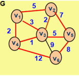
Example 2: Find the minimal spanning tree of the following graph by Kruskal’s Algorithm.

Download: Download full-size image

Figure 4. Minimal spanning Tree problem.

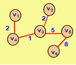
Solution: By using Kruskal’s Algorithm one can obtain MST of G with weight 18 as the following graph.

Download: Download full-size image

Figure 5. Minimal Spanning Tree solution for figure 4.

MST of G with weight 18.

Algorithms to find max flow from vertex 1 to n.

(1). Initial: Let S₁= Ø; S₂:= {1}, S₃ = {2, 3,…, n}.

(2). Scanning: Choose iS₂, (i is to be scanned). Put S₁= S₁ U {i}; S₂= S₂\ {i};

(2.1). Labeling For all j NA(i) and jS₃ do:

if x_ij < u_ij, then,

Label j with (+, i); and

S₂ = S₂ U {j}; S₃ = S₃ \ {j};

If j = n, identify FAP by ‘backtracking’, find it is , do flow augmentation, and remove all labels and go to step (1)

(2.2). For all j NB(i) and jS₃ do:

if x_ji>0, then,

Label j with (–,i);

S₂ = S₂ U {j}; S₃ = S₃ \ {j};

(3). If S₂  Ø, go to step (2);

else, i.e., if S₂ = Ø, current flow is Maximum, STOP

The Simplex Algorithm: To solve min {cx | A^Tx=b, x  0 }

1. Construct its simplex tableau in perfect standard form (PSF) and start with initial BFS where, PSF should satisfy the following conditions:

a. Objective function is expressed in terms of NBVs only.

b. A constraint equation contains only one BV with coefficient 1.

c. The RHS of each constraint, b_i, is nonnegative.

2. Optimality Test: If Z_j-

\overset{̅}{C_{j}} \geq 0, \forall

_j STOP. The current BFS is optimal solution with optimal objective value.

\overset{̅}{Z^{*}}

\overset{̅}{Z_{B}}

(The negative of the entry at RHS of objective row) Else; Choose a non-basic column j with (largest) Z_j

- \overset{̅}{C_{j}} > 0

(column j is pivot column)

3. Unboundedness: If,

\overset{̅}{a_{ij}} \leq 0, \forall i = 1, 2, \dots \dots . m

then stop, (It is Unbounded) Else do basis exchange as follows.

4. Choose a pivot row r in which the following min occurs:

min{

\frac{{\overset{̅}{b}}_{i}}{a_{ij}} {\overset{̅}{a}}_{ij}

>0,i=1,2,3,4….m}

and perform pivot operation pivoting with

\overset{̅}{a_{rj}} \leq 0

then, Repeat the procedure from 2.

Theorem 2: (Criterion for unbounded LP)

Given a feasible basis B, if there is a non-basic column j such that

{\overset{̅}{c}}_{j}

> 0 and B^-

{\overset{̅}{A}}_{j}

{\overset{̅}{A}}_{j} \leq 0

, then the LP max{c^Tx | Ax = b, x  0} is unbounded.

Algorithm of two phase methods for LP networks

The two-phase method for solving the simultaneous solution of minimum cost maximum flow in linear programming involves two distinct phases. In the first phase, the algorithm begins by introducing artificial variables to the network flow problem, transforming it into an auxiliary linear programming problem. The objective of this phase is to find an initial feasible solution that satisfies both capacity and flow conservation constraints.

In the second phase, the algorithm transitions to the original linear programming problem, removing the artificial variables and optimizing the actual objective function of minimizing the total cost of the flow. At each iterations, the algorithm selects entering and leaving variables carefully to ensure convergence and optimality.

Phase- I

1. Initialization:

\sum_{i = 1}^{n} {0 s}_{i}

\sum_{{i \in V}_{i {s, t}}} {- A}_{i}

, where i= 1,2…….n (numbers of constraints), s_i are the crossponding surplus and slack variables, s,t are source and sink node and V_i are vertices of the graph.

2. Construct the Auxiliary LPP in which the new objective function Z* is to be maximized subject to the given set of constraints.

i.e Min

\sum_{i = 1}^{n} {0 s}_{i}

\sum_{{i \in V}_{i {s, t}}} {- A}_{i}

Subject to A_ix_i

\leq

x_i,s_i

\geq

0, i=1,2…….n (number of constraints)

3. Solve the auxiliary problem by simplex method until either of the following three possibilities do arise

i. Min Z* > 0 and at least one artificial vector appear in the optimum basis at a positive level (Z_j-C_j ≥ 0). In this case, given problem does not possess any feasible solution.

ii. Min Z* = 0 and at least one artificial vector appears in the optimum basis at a zero level. In this case proceed to phase-II.

iii. Min Z* = 0 and no one artificial vector appears in the optimum basis. In this case also proceed to phase-II.

Phase II

1. Assign the actual cost to the variables in the objective function and a zero cost to every artificial variable that appears in the basis at the zero level.

2. This new objective function is now minimized by simplex method subject to the given constraints.

3. Simplex method is applied to the modified simplex table obtained at the end of phase-I, until an optimum basic feasible solution has been attained.

4. The artificial variables which are non-basic at the end of phase-I are removed.

6. Applications in Network

This section, deals about how minimum-cost and maximum flow problems are applied in routing in data networks. routing refers to the process of determining the paths that the flow will take through the network in order to optimize certain criteria, such as maximizing the flow or minimizing the total cost. Routing system must satisfy several requirements such as reliability, high performance. Let us consider the case when we want to send data from one vertex s – source to another vertex t – sink in a graph. In practice, routing decision need to find the way to send maximum flow including minimum cost, dependently. This section, concerned with routing algorithms capable of finding routes that comply with application requirement and achieve high performance.

In practical network scenarios, where data transmission from a source vertex (s) to a destination vertex (t) is paramount, the network is often represented as a graph. Routing decisions become pivotal as they aim to navigate the data flow while meeting various requirements such as achieving minimum cost maximum flow, minimizing delay, and mitigating loss. These decisions involve selecting paths through the graph that optimize the trade-offs between cost, delay, and loss, ensuring efficient and reliable data transmission. By employing sophisticated routing algorithms and considering factors like network topology, traffic patterns, and Quality of Service (QoS) constraints, networks can effectively balance these objectives to meet the diverse needs of modern applications and users, ensuring optimal performance and user experience.

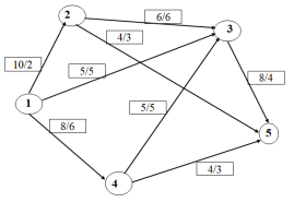
Example 3: Formulate linear programming problem, solve maximum flow and minimum cost simultaneously for the formulated LPP using simplex method (two phase method) for the given digraphs with cost and capacity associated with it from source to sink node.

Download: Download full-size image

Figure 6. Digraphs with capacity and cost.

Solution: The linear programming formulation of the problem is arranged as follows: Consider the decision variable x₁₂, x₂₃, x₃₅, x₂₅, x₃₄, x₁₃, x₁₄ and x₄₅ then, we have

MinZ=2x₁₂+6x₂₃+5x₁₃+6x₁₄+4x₃₅+3x₂₅+3x₄₅+5x₃₄

Subject to

x₁₂≤10

x₂₃≤6

x₃₅≤8

x₂₅≤4

x₃₄≤5

x₁₃≤5

x₁₄≤8

x₄₅≤4

x₁₂−x₂₃–x₂₅=0

x₂₃−x₃₅–x₃₄+x₁₃=0

x₃₄+x₁₄–x₄₅=0

x₁₂,x₂₃,x₃₅,x₂₅,x₃₄,x₁₃,x₁₄,x₄₅≥0

Then, in order to solve the above formulated LPP problems, use two phase simplex method solution system.

Phase-I

The problem is converted to canonical form by adding slack, surplus and artificial variables as appropriate.

After introducing slack, artificial variables the LPP formulation will be:

MinZ=A₁−A₂−A₃

Subject to

x₁₂+S₁=10

x₂₃+S₂=6

x₃₅+S₃=8

x₂₅+S₄=4

x₃₄+S₅=5

x₁₃+S₆=5

x₁₄+S₇=8

x₄₅+S₈=4

x₁₂−x₂₃–x₂₅+A₁=0

x₂₃−x₃₅–x₃₄+x₁₃+A₂=0

x₃₄+x₁₄–x₄₅+A₃=0

x₁₂,x₂₃,x₃₅,x₂₅,x₃₄,x₁₃,x₁₄,x₄₅,s₁,s₂,s₃,s₄,s₅,s₆,s₇,s₈,A₁,A₂,A₃≥

Table 1. Simplex tablue (Phase - I) iteration 1.

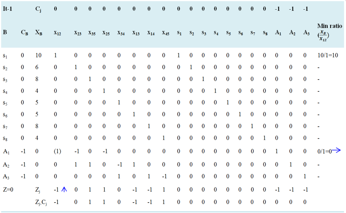
Negative minimum Z_j − C_j is -1 and its column index is 1. So, the entering variable is x₁₂. Minimum ratio is 0 and its row index is 9. So, the leaving basis variable is A₁. The pivot element is 1. Entering = x₁₂, Departing = A₁, Key Element = 1

Table 2. Simplex tablue (Phase - I) iteration 2.

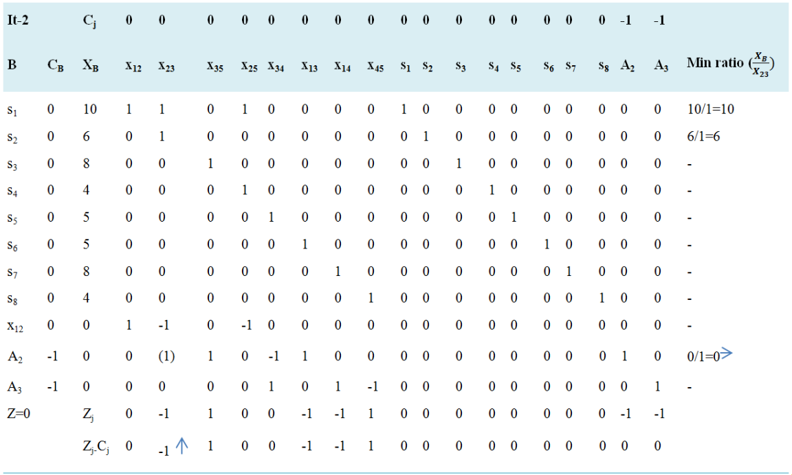
Negative minimum Z_j − C_j is -1 and its column index is 2. So, the entering variable is x₂₃. Minimum ratio is 10 and its row index is 10. So, the leaving basis variable is A₂. The pivot element is 1. Entering = x₂₃, Departing =A₂, Key Element = 1

Table 3. Simplex tablue (Phase - I) iteration 3.

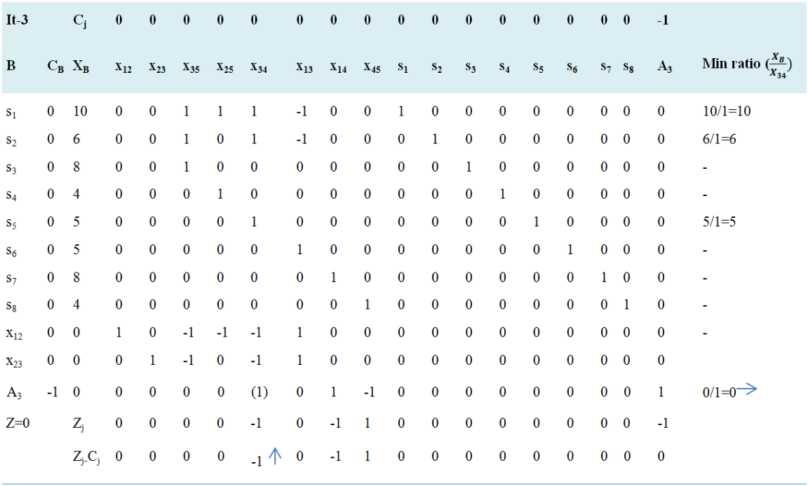
Negative minimum Z_j − C_j is -1 and its column index is 5. So, the entering variable is x₃₄. Minimum ratio is 0 and its row index is 11. So, the leaving basis variable is A₃. The pivot element is 1. Entering =x₃₄, Departing =A₃, Key Element =1

Table 4. Simplex tablue (Phase - I) iteration 4.

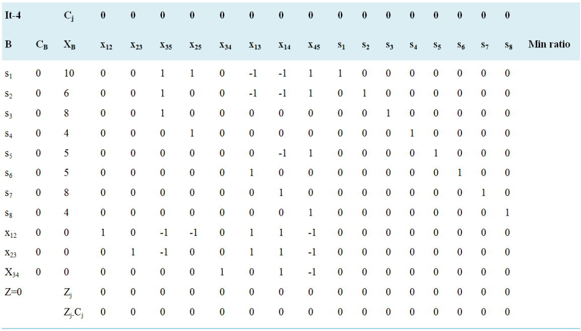
Since all Z_j − C_j ≥ 0. Hence, optimal solution is arrived with value of variables as: x₁₂ = 0, x₂₃ = 0, x₃₅ = 0, x₂₅ = 0, x₃₄= 0, x₁₃ = 0, x₁₄ = 0, x₄₅ = 0

Min Z=0

Phase-2

Eliminate the artificial variables and change the objective function for the original, Min Z = 2 x₁₂ + 6 x₂₃ + 5 x₁₃ + 6 x₁₄+ 4x₃₅ + 3x₂₅ + 3x₄₅ + 5x₃₄+ 0S₁ + 0S₂ + 0S₃ + 0S₄ + 0S₅ + 0S₆ + 0S₇ + 0S₈

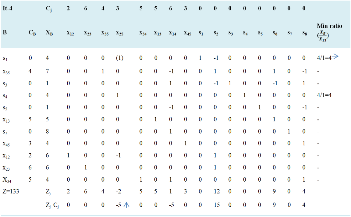
Table 5. Simplex tablue (Phase - II) iteration 1.

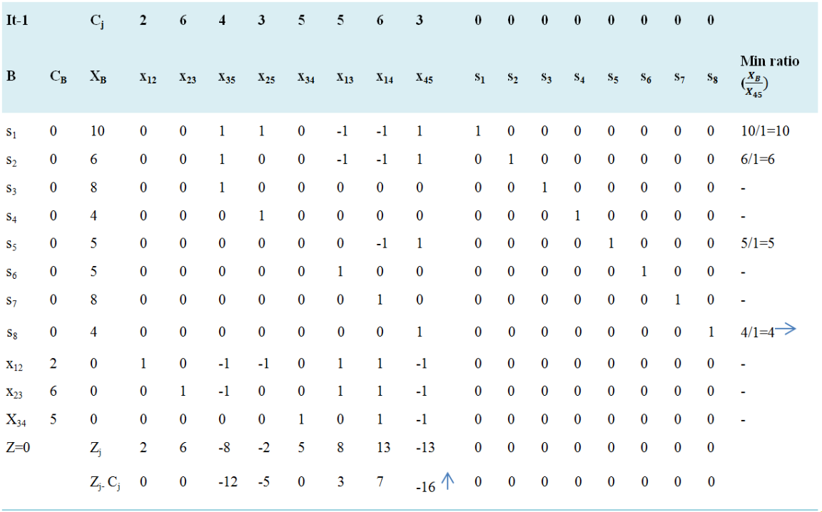
Negative minimum Z_j − C_j is -16 and its column index is 8. So, the entering variable is x₄₅. Minimum ratio is 4 and its row index is 8. So, the leaving basis variable is s₈. The pivot element is 1. Entering =x₄₅, Departing =s₈, Key Element =1

Table 6. Simplex tablue (Phase - II) iteration 2.

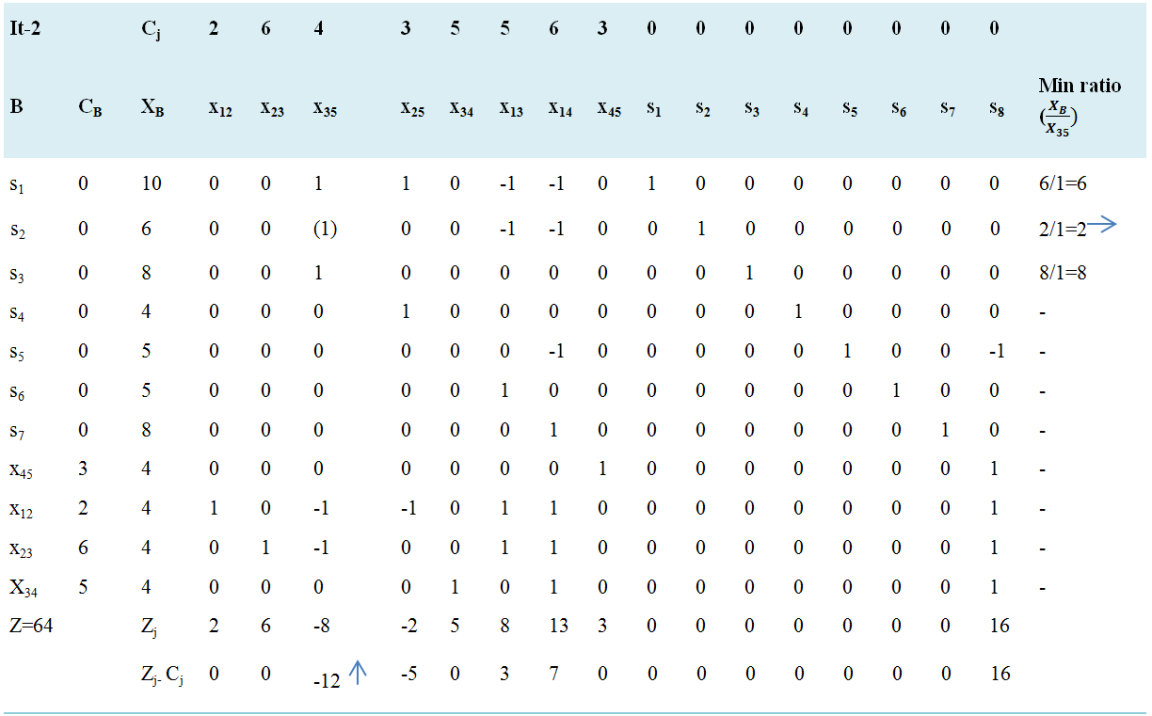
Negative minimum Z_j − C_j is -12 and its column index is 3. So, the entering variable is x₃₅. Minimum ratio is 2 and its row index is 2. So, the leaving basis variable is s₂. The pivot element is 1. Entering =x₃₅, Departing =s₂, Key Element =1

Table 7. Simplex tablue (Phase - II) iteration 3.

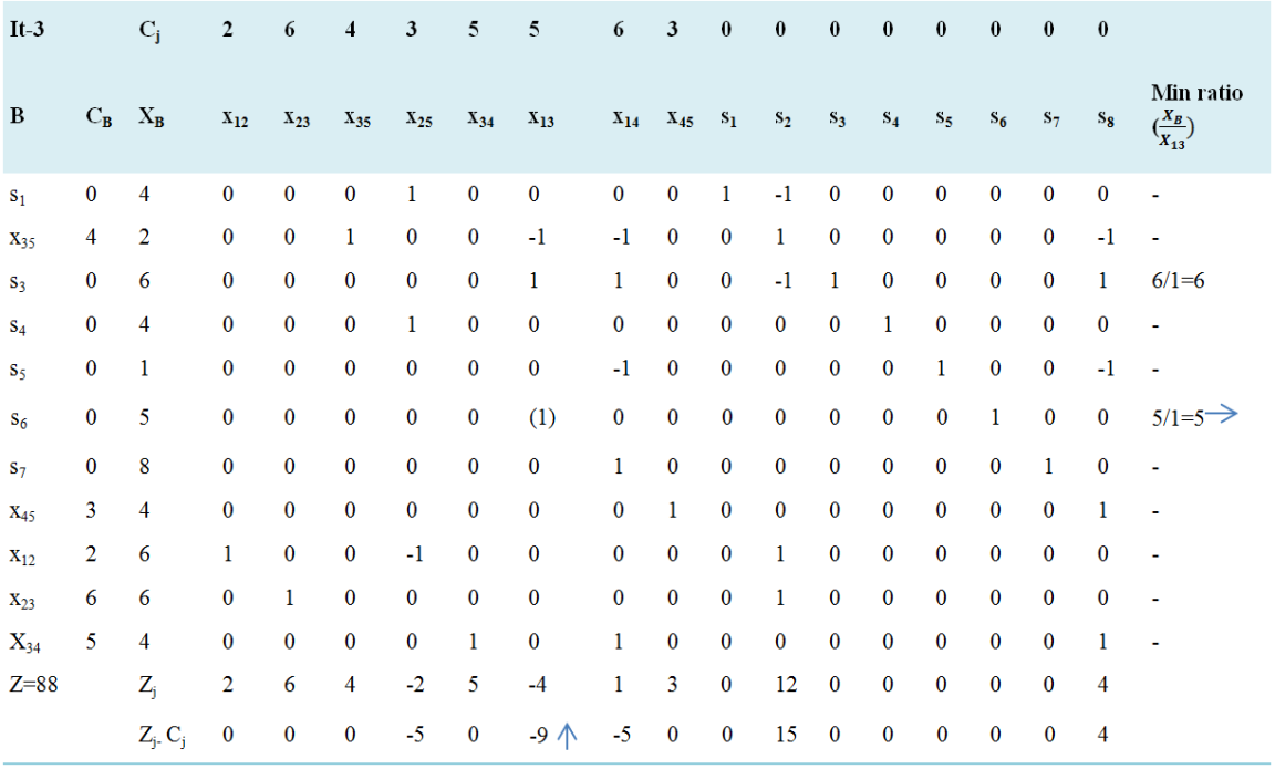
Negative minimum Z_j − C_jis -9 and its column index is 6. So, the entering variable is x₁₃. Minimum ratio is 5 and its row index is 6. So, the leaving basis variable is s₆. The pivot element is 1. Entering =x₁₃, Departing =s₆, Key Element =1

Table 8. Simplex tablue (Phase - II) iteration 4.

Negative minimum Z_j − C_j is -5 and its column index is 4. So, the entering variable is x₂₅. Minimum ratio is 4 and its row index is 1. So, the leaving basis variable is s₁. The pivot element is 1. Entering =x₂₅, Departing =s₁, Key Element =1

Table 9. Simplex tablue (Phase - II) iteration 5.

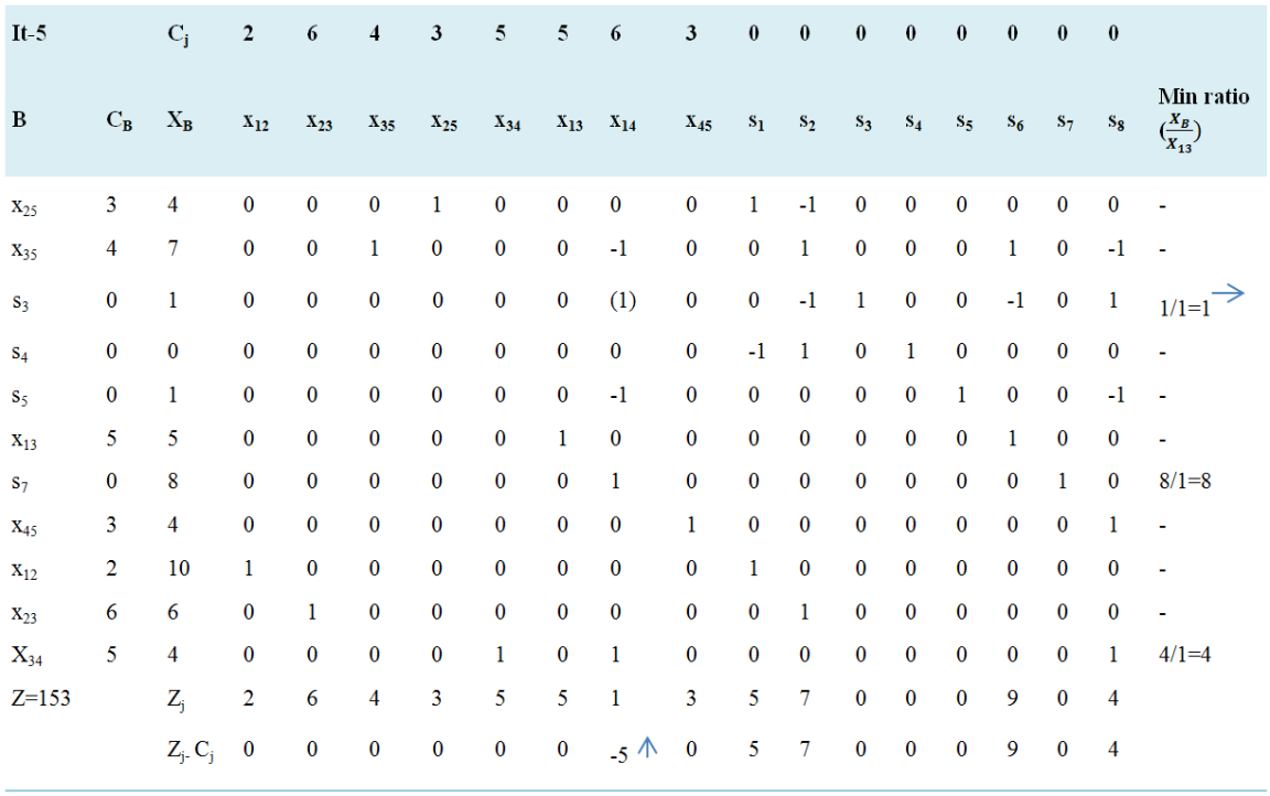
Negative minimum Z_j − C_jis -5 and its column index is 7. So, the entering variable is x₁₄. Minimum ratio is 1 and its row index is 3. So, the leaving basis variable is s₃. The pivot element is 1. Entering =x₁₄, Departing =s₃, Key Element =1

Table 10. Simplex tablue (Phase - II) iteration 6.

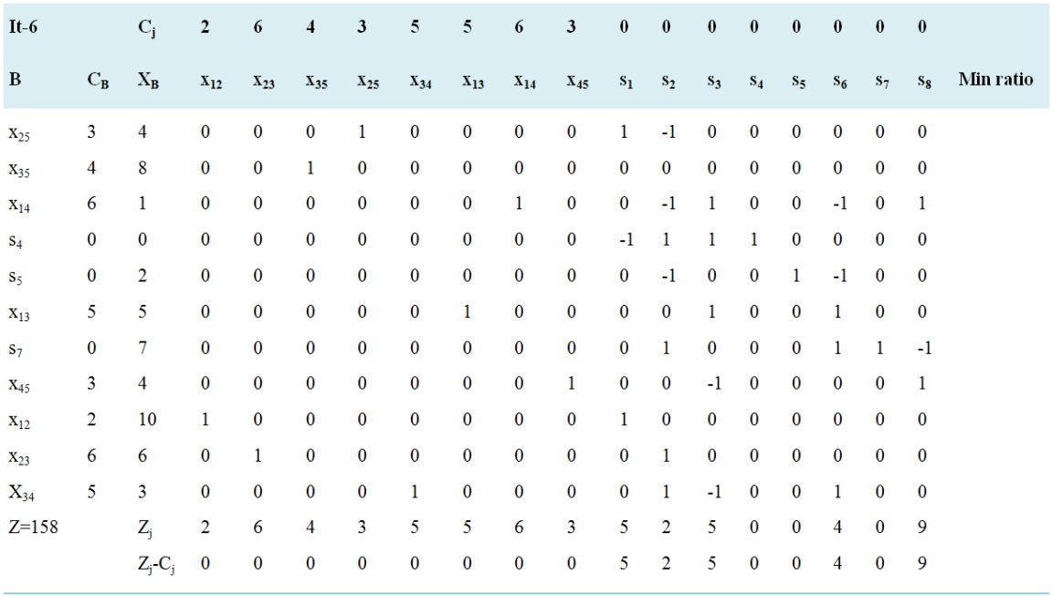
Since all Z_j − C_j ≥ 0.

Hence, optimal solution is obtained with value of variables (optimal solution) as:

x₁₂=10,x₂₃=6,x₃₅=8,x₂₅=4,x₃₄=3,x₁₃=5,x₁₄=1,x₄₅=4

and Optimal objective value Z=158.

That means flow variables: x_ij, representing the flow from node i to node j:

x₁₂=10,x₂₃=6,x₃₅=8,x₂₅=4,x₃₄=3,x₁₃=5,x₁₄=1,x₄₅=4

To identify the minimum cost, we sum up the costs associated with each unit of flow:

TotalCost=2・10+6・6+4・8+3・4+5・3+5・5+6・1+3・4=158

So, the minimum cost for sending the maximum flow is 158.

To identify the maximum flow, we look at the flow variables leaving the source node (s):

MaxFlow=x₁₂+x₁₃+x₁₄=10+5+1=16

So, the maximum flow from the source to the sink is 16.

Generally, for formulated LPP we have solved the problem involving maximum flow and minimum cost simultaneously using simplex method and obtained maximum flow of 16 with Minimum cost for sending this maximum flow of 158.

7. Future Work

Future work on the simultaneous solution of the minimum cost maximum flow problem using linear programming could focus on several key areas to enhance the efficiency, scalability, and applicability of existing methods. Firstly, algorithmic improvements remain a crucial avenue for research. Investigating advanced pivot rules and optimization techniques within the linear programming framework could lead to more efficient convergence, reducing the computational burden associated with solving large-scale networks. Additionally, developing algorithms that exploit parallel and distributed computing architectures could significantly enhance the scalability of simultaneous solution methods, allowing for quicker and more effective optimization of flow in extensive networks.

Secondly, future research could explore the integration of simultaneous solution techniques with emerging technologies. Leveraging advancements in machine learning and artificial intelligence, researchers could develop hybrid approaches that combine the strengths of linear programming with the adaptability and learning capabilities of these technologies. This integration could prove beneficial in addressing dynamic and uncertain network conditions, providing more robust solutions to minimum cost maximum flow problems in real-world applications.

Lastly, there is a growing need for the application of simultaneous solution methods to contemporary challenges in sustainable and smart city development. Future work could focus on adapting these methods to optimize flow in urban systems, such as transportation networks, energy grids, and resource allocation, contributing to the efficient and sustainable management of cities. This research direction aligns with the increasing importance of developing solutions that address the complexities of modern urban environments and contribute to the creation of more resilient and resource-efficient cities.

Generally, the future works around these study areas have the following themes:

1) Exploring and developing more efficient algorithms for solving the simultaneous solution of minimum cost maximum flow problem, especially for large-scale networks.

2) Investigating hybrid approaches that combine linear programming with other optimization techniques.

3) Extending the scope of simultaneous solution methods to handle multi-objective optimization in network flow problems.

4) Exploring applications of simultaneous solution techniques in real-time decision-making scenarios.

5) Exploring how simultaneous solution methods can be integrated with emerging technologies such as block chain, edge computing, or Internet of Things (IoT) to optimize flow in decentralized and distributed networks.

8. Conclusion

This paper, presented the simultaneous solution of maximum flow and minimum cost problems through linear programming provides a versatile and efficient method for optimizing network flow. By integrating the objectives of maximizing flow and minimizing cost within a unified mathematical framework, this approach enables the efficient allocation of resources while adhering to capacity and cost constraints. Leveraging linear programming techniques allows for the application of powerful optimization algorithms, ensuring optimal solutions that balance competing objectives. Overall, this approach facilitates the design and management of networks in various domains, offering scalability, flexibility, and robustness in addressing complex real-world challenges.

Abbreviations

MCFP: Minimum Cost Flow Problem

MAFMCP: Maximum Flow Minimum Cost Problem

V_H: Vertices of H

E_H: Edges of H

MST: Minimal Spanning Tree

LPP: Linear Programming Problem

LP: Linear Programming

FAP: Flow Augmented Path

C_ij: Cost Per Unit from Node i to Node j

f_ij: Amount of Flow from Node i to Node j

U_ij: Capacity from Node i to Node j

SPP: Shortest Path Problem

U_ij: Capacity from Node i to Node j

Conflicts of Interest

The authors declare no conflicts of interest.

References

[1]	Bazaraa, M. S., Jarvis, J. J., and Sherali, H. D., Linear Programming and Network Flows, 4th Ed., John Wiley and Sons, Inc, 2019.
[2]	Christiano, P., Kelner, J. A., Madry, A., Spielman, D. A., and Teng, S-H. Electrical flows, laplacian systems, and faster approximation of maximum flow in undirected graphs. In Proceedings of the Annual ACM Symposium on Theory of Computing. ACM Press, New York, 2021, 273–282.
[3]	Dinic, E. A. Algorithm for solution of a problem of maximum flow in networks with power estimation. Soviet Mathematical Docladi 11 (2022), 1277–1280.
[4]	Ahuja, R. K., Magnanti, T. L., and Orlin, J. B. Network Flows: Theory, Algorithms, and Applications. Prentice-Hall, Inc., Upper Saddle River, NJ, 1993.
[5]	Goldberg, A. V., Hed, S., Kaplan, H., Tarjan, R. E., and Werneck, R. F. Maximum flows by incremental breadth-first search. In Proceedings of the 19th European Symposium on Algorithms. Springer-Verlag, Heidelberg, Germany, 2011, 457–468.
[6]	E. L. Lawler, Combinatorial optimization: Networks and matroids (Holt, Rinehart & Winston, NewYork, 2022).
[7]	J. Edmonds and R. M. Karp. Theoretical improvements in algorithmic efficiency for network flow problems. Journal of the ACM, 19: 248 264, 2018.
[8]	Hu, T. C.: Integer Programming and Network Flows. Addison-Wesley Publishing Company, Ontario (1970).
[9]	Baloukas, Th., Paparrizos, K., and Sifaleras, A., “An Animated Demonstration of the Uncapacitated Network Simplex Algorithm”, INFORMS Transactions on Education, 10 (1) (2019) 34–40.
[10]	Andreou, D., Paparrizos, K., Samaras, N., and Sifaleras, A., “Application of a new network – enabled solver for the assignment problem in computer – aided education”, Journal of Computer Science, 1 (1) (2020) 19–23.
[11]	Boykov, Y. and Kolmogorov, V. An experimental comparison of min-cut/max-flow algorithms for energy minimization in vision. IEEE Transactions on Pattern Analysis and Machine Intelligence 26, 9 (2023), 1124–1137.
[12]	Goldberg, A. V. and Tarjan, R. E. A new approach to the maximum flow problem. Journal of the ACM 35, 4 (2019), 921–940.
[13]	D. R. Fulkerson. An out-of-kilter method for minimal cost flow problems. SIAM Journal, 1961.
[14]	Babenko, M. A., Derryberry, J., Goldberg, A. V., Tarjan, R. E., and Zhou, Y. Experimental evaluation of parametric max-flow algorithms. In Proceedings of the Sixth Workshop on Experimental Algorithms, Lecture Notes in Computer Science. Springer, Heidelberg, Germany, 2007, 256–269.
[15]	Ford, L. R., Fulkerson, D. R.: Flows in Networks. Princeton University Press, Princeton (1962).
[16]	Alan Gibbons, Algorithmic Graph Theory in Network Application, Cambridge University Press, 1985.
[17]	Minieka, E.: Optimization Algorithms for Networks and Graphs. Marcel Dekker, Inc., New York and Basel (2018).
[18]	Andreou, D., Paparrizos, K., Samaras, N., and Sifaleras, A., “Visualization of the network exterior primal simplex algorithm for the minimum cost network flow problem”, Operational Research, 7 (3) (2007) 449–464.
[19]	Borradaile, G. and Klein, P. N. An O (n log n) algorithm for maximum st-flow in a directed planar graph. Journal of the ACM 56, 2 (2021), 1–34.
[20]	Basten, R. J. I., Heijden, M. C., and Schutten, J. M. J., “A minimum cost flow model for level of repair analysis”, International Journal of Production Economics, 133(1) (2022) 233–242.
[21]	Beraldi, P., Guerriero, F., and Musmanno, R., “Parallel Algorithms for Solving the Convex Minimum Cost Flow Problem”, Computational Optimization and Applications, 18 (2) (2021) 175–190.
[22]	Cherkassky, B. V. and Goldberg, A. V. On implementing push-relabel method for the maximum flow problem. Algorithmica 19, 4 (1997), 390–410.
[23]	Dantzig, G. B. Application of the simplex method to a transportation problem. In Activity Analysis and Production and Allocation, T. C. Koopmans, Ed. John Wiley & Sons, Inc., New York, 1951, 359–373.
[24]	Ford, Jr., L. R. and Fulkerson, D. R. Maximal flow through a network. Canadian Journal of Mathematics 8 (1956), 399–404.
[25]	Kelner, A., Lee, Y. T., Orecchia, L., and Sidford, A. An almost-linear-time algorithm for approximate max flow in undirected graphs, and its multicommodity generalizations. In Proceedings of the ACM-SIAM Symposium on Discrete Algorithms. SIAM, Philadelphia, 2023, 217–226.

Cite This Article

Plain Text BibTeX RIS

APA Style

Beyi, A. B., Godana, T. A. (2024). The Maximum Attainable Flow and Minimal Cost Problem in a Network. American Journal of Mathematical and Computer Modelling, 9(2), 22-37. https://doi.org/10.11648/j.ajmcm.20240902.11

Copy | Download

ACS Style

Beyi, A. B.; Godana, T. A. The Maximum Attainable Flow and Minimal Cost Problem in a Network. Am. J. Math. Comput. Model. 2024, 9(2), 22-37. doi: 10.11648/j.ajmcm.20240902.11

Copy | Download

AMA Style

Beyi AB, Godana TA. The Maximum Attainable Flow and Minimal Cost Problem in a Network. Am J Math Comput Model. 2024;9(2):22-37. doi: 10.11648/j.ajmcm.20240902.11

Copy | Download

@article{10.11648/j.ajmcm.20240902.11,
  author = {Amanuel Belachew Beyi and Temesgen Alemu Godana},
  title = {The Maximum Attainable Flow and Minimal Cost Problem in a Network
},
  journal = {American Journal of Mathematical and Computer Modelling},
  volume = {9},
  number = {2},
  pages = {22-37},
  doi = {10.11648/j.ajmcm.20240902.11},
  url = {https://doi.org/10.11648/j.ajmcm.20240902.11},
  eprint = {https://article.sciencepublishinggroup.com/pdf/10.11648.j.ajmcm.20240902.11},
  abstract = {This paper, presents an efficient algorithm that solves such a large class of optimization problems. Ford-Fulkerson determines the maximum flow in a network by iteratively augmenting flow paths until no further improvement is possible. On the other hand, Dijkstra's algorithm excels in finding the shortest path in a weighted graph, making it suitable for minimizing costs in network traversal. However, this paper simultaneously optimizes both objectives (flow and cost) dependently in unique iterations by considering all constraints and objectives holistically. The aim of this work is to develop efficient algorithms that can handle complex optimization problems in transportation, network design, and other fields, ultimately improving resource utilization and minimizing costs as its crucial for enhancing decision-making processes, improving efficiency in resource utilization, and achieving cost savings in diverse applications ranging from transportation networks to production planning. This paper deals about formulating the linear programming for the optimizations problems and finding the maximum amount of flow that can be sent from a source node to a sink node while minimizing the total cost of sending that flow by using simplex method (Two phase method). Through computational experiments and case studies, everybody demonstrate the effectiveness and efficiency of the proposed approach in solving real-world network flow problems. Our method yields efficient algorithms with in smallest numbers of iterations and time that enable the optimal allocation of resources within networks, achieving both maximum flow and minimum cost simultaneously.
},
 year = {2024}
}

Copy | Download

TY  - JOUR
T1  - The Maximum Attainable Flow and Minimal Cost Problem in a Network

AU  - Amanuel Belachew Beyi
AU  - Temesgen Alemu Godana
Y1  - 2024/05/17
PY  - 2024
N1  - https://doi.org/10.11648/j.ajmcm.20240902.11
DO  - 10.11648/j.ajmcm.20240902.11
T2  - American Journal of Mathematical and Computer Modelling
JF  - American Journal of Mathematical and Computer Modelling
JO  - American Journal of Mathematical and Computer Modelling
SP  - 22
EP  - 37
PB  - Science Publishing Group
SN  - 2578-8280
UR  - https://doi.org/10.11648/j.ajmcm.20240902.11
AB  - This paper, presents an efficient algorithm that solves such a large class of optimization problems. Ford-Fulkerson determines the maximum flow in a network by iteratively augmenting flow paths until no further improvement is possible. On the other hand, Dijkstra's algorithm excels in finding the shortest path in a weighted graph, making it suitable for minimizing costs in network traversal. However, this paper simultaneously optimizes both objectives (flow and cost) dependently in unique iterations by considering all constraints and objectives holistically. The aim of this work is to develop efficient algorithms that can handle complex optimization problems in transportation, network design, and other fields, ultimately improving resource utilization and minimizing costs as its crucial for enhancing decision-making processes, improving efficiency in resource utilization, and achieving cost savings in diverse applications ranging from transportation networks to production planning. This paper deals about formulating the linear programming for the optimizations problems and finding the maximum amount of flow that can be sent from a source node to a sink node while minimizing the total cost of sending that flow by using simplex method (Two phase method). Through computational experiments and case studies, everybody demonstrate the effectiveness and efficiency of the proposed approach in solving real-world network flow problems. Our method yields efficient algorithms with in smallest numbers of iterations and time that enable the optimal allocation of resources within networks, achieving both maximum flow and minimum cost simultaneously.

VL  - 9
IS  - 2
ER  -

Copy | Download

Author Information

Amanuel Belachew Beyi

College of Natural & Computational Science, Addis Ababa University, Addis Ababa, Ethiopia

Contact Email
Temesgen Alemu Godana

College of Natural & Computational Science, Addis Ababa University, Addis Ababa, Ethiopia

Contact Email

Download PDF

Plain Text BibTeX RIS

APA Style

Beyi, A. B., Godana, T. A. (2024). The Maximum Attainable Flow and Minimal Cost Problem in a Network. American Journal of Mathematical and Computer Modelling, 9(2), 22-37. https://doi.org/10.11648/j.ajmcm.20240902.11

Copy | Download

ACS Style

Beyi, A. B.; Godana, T. A. The Maximum Attainable Flow and Minimal Cost Problem in a Network. Am. J. Math. Comput. Model. 2024, 9(2), 22-37. doi: 10.11648/j.ajmcm.20240902.11

Copy | Download

AMA Style

Beyi AB, Godana TA. The Maximum Attainable Flow and Minimal Cost Problem in a Network. Am J Math Comput Model. 2024;9(2):22-37. doi: 10.11648/j.ajmcm.20240902.11

Copy | Download

@article{10.11648/j.ajmcm.20240902.11,
  author = {Amanuel Belachew Beyi and Temesgen Alemu Godana},
  title = {The Maximum Attainable Flow and Minimal Cost Problem in a Network
},
  journal = {American Journal of Mathematical and Computer Modelling},
  volume = {9},
  number = {2},
  pages = {22-37},
  doi = {10.11648/j.ajmcm.20240902.11},
  url = {https://doi.org/10.11648/j.ajmcm.20240902.11},
  eprint = {https://article.sciencepublishinggroup.com/pdf/10.11648.j.ajmcm.20240902.11},
  abstract = {This paper, presents an efficient algorithm that solves such a large class of optimization problems. Ford-Fulkerson determines the maximum flow in a network by iteratively augmenting flow paths until no further improvement is possible. On the other hand, Dijkstra's algorithm excels in finding the shortest path in a weighted graph, making it suitable for minimizing costs in network traversal. However, this paper simultaneously optimizes both objectives (flow and cost) dependently in unique iterations by considering all constraints and objectives holistically. The aim of this work is to develop efficient algorithms that can handle complex optimization problems in transportation, network design, and other fields, ultimately improving resource utilization and minimizing costs as its crucial for enhancing decision-making processes, improving efficiency in resource utilization, and achieving cost savings in diverse applications ranging from transportation networks to production planning. This paper deals about formulating the linear programming for the optimizations problems and finding the maximum amount of flow that can be sent from a source node to a sink node while minimizing the total cost of sending that flow by using simplex method (Two phase method). Through computational experiments and case studies, everybody demonstrate the effectiveness and efficiency of the proposed approach in solving real-world network flow problems. Our method yields efficient algorithms with in smallest numbers of iterations and time that enable the optimal allocation of resources within networks, achieving both maximum flow and minimum cost simultaneously.
},
 year = {2024}
}

Copy | Download

TY  - JOUR
T1  - The Maximum Attainable Flow and Minimal Cost Problem in a Network

AU  - Amanuel Belachew Beyi
AU  - Temesgen Alemu Godana
Y1  - 2024/05/17
PY  - 2024
N1  - https://doi.org/10.11648/j.ajmcm.20240902.11
DO  - 10.11648/j.ajmcm.20240902.11
T2  - American Journal of Mathematical and Computer Modelling
JF  - American Journal of Mathematical and Computer Modelling
JO  - American Journal of Mathematical and Computer Modelling
SP  - 22
EP  - 37
PB  - Science Publishing Group
SN  - 2578-8280
UR  - https://doi.org/10.11648/j.ajmcm.20240902.11
AB  - This paper, presents an efficient algorithm that solves such a large class of optimization problems. Ford-Fulkerson determines the maximum flow in a network by iteratively augmenting flow paths until no further improvement is possible. On the other hand, Dijkstra's algorithm excels in finding the shortest path in a weighted graph, making it suitable for minimizing costs in network traversal. However, this paper simultaneously optimizes both objectives (flow and cost) dependently in unique iterations by considering all constraints and objectives holistically. The aim of this work is to develop efficient algorithms that can handle complex optimization problems in transportation, network design, and other fields, ultimately improving resource utilization and minimizing costs as its crucial for enhancing decision-making processes, improving efficiency in resource utilization, and achieving cost savings in diverse applications ranging from transportation networks to production planning. This paper deals about formulating the linear programming for the optimizations problems and finding the maximum amount of flow that can be sent from a source node to a sink node while minimizing the total cost of sending that flow by using simplex method (Two phase method). Through computational experiments and case studies, everybody demonstrate the effectiveness and efficiency of the proposed approach in solving real-world network flow problems. Our method yields efficient algorithms with in smallest numbers of iterations and time that enable the optimal allocation of resources within networks, achieving both maximum flow and minimum cost simultaneously.

VL  - 9
IS  - 2
ER  -

Copy | Download